
Uncertainty#
Bootstrap Resampling#
Bootstrap resampling repeatedly samples data with replacement to estimate uncertainty and build confidence intervals without relying on parametric assumptions.
Steps:
Start with an original dataset of size \( n \):
\[ X = [1, 2, 3, 4, 5, 6, 7, 8, 9] \]Resample with replacement:
\[ X^*_1 = [1, 9, 2, 5, 4],\quad X^*_2 = [3, 3, 5, 8, 1],\quad X^*_3 = [7, 5, 9, 2, 4] \]Calculate the desired statistic (e.g., mean) for each bootstrap sample.
\[ \bar{X}_1^* = 5.8,\quad \bar{X}_2^* = 4.6,\quad \bar{X}_3^* = 5.2 \]Repeat steps 2–3, typically thousands of times, generating an empirical distribution for the statistic.
Use the bootstrap distribution to estimate uncertainty, confidence intervals, standard errors, or bias of the statistic.
Tips:
Quality and representativeness of bootstrap estimates depend heavily on the original dataset.
Can underestimate uncertainty or fail to accurately represent the sampling distribution when data is highly skewed, contains outliers, or has strong dependence structures (time series, spatial data).
Interpret bootstrap results carefully—especially with complex or highly correlated data.
import numpy as np
import matplotlib.pyplot as plt

def bootstrap_mean(data, n_bootstrap=10000, random_state=44):
    """Performs bootstrap resampling to estimate mean confidence intervals.

    Args:
        data: Original sample data (array-like).
        n_bootstrap: Number of bootstrap samples to generate.
        random_state: Seed for reproducibility.

    Returns:
        Array of bootstrap means.
    """
    rng = np.random.default_rng(random_state)
    sample_indices = rng.integers(0, len(data), size=(n_bootstrap, len(data)))
    return data[sample_indices].mean(axis=1)


data = np.array([1, 2, 3, 4, 5, 6, 7, 8, 9, 10])
bootstrap_means = bootstrap_mean(data, n_bootstrap=10000, random_state=44)
ci_lower, ci_upper = np.percentile(bootstrap_means, [2.5, 97.5])

print(f"Bootstrap Mean Estimate: {np.mean(bootstrap_means):.2f}")
print(f"95% Confidence Interval: [{ci_lower:.2f}, {ci_upper:.2f}]")

fig, axes = plt.subplots(1, 2, figsize=(10, 3), constrained_layout=True)

# Original Data Distribution
axes[0].hist(data, edgecolor='k', alpha=0.7)
axes[0].set_title("Original Data Distribution")
axes[0].set_xlabel("Values")
axes[0].set_ylabel("Frequency")

# Bootstrap Distribution of the Mean
axes[1].hist(bootstrap_means, bins=30, edgecolor='k', alpha=0.7)
axes[1].axvline(ci_lower, color='tab:olive', linestyle='--', label='95% CI Lower')
axes[1].axvline(ci_upper, color='tab:purple', linestyle='--', label='95% CI Upper')
axes[1].set_title("Bootstrap Distribution of the Mean")
axes[1].set_xlabel("Mean Values")
axes[1].set_ylabel("Frequency")
axes[1].legend()

plt.show()
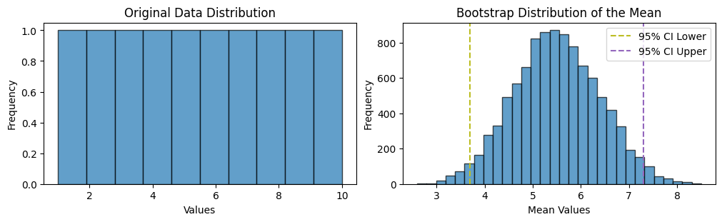
Bootstrap Mean Estimate: 5.49
95% Confidence Interval: [3.70, 7.30]
rng = np.random.default_rng(42)
sample_indices = rng.integers(0, len(data), size=(10, len(data)))
data_treatments = data[sample_indices]

# Compute bootstrap means and CIs
means_control = bootstrap_mean(data, n_bootstrap=1000, random_state=42)
mean_control = means_control.mean()

means_treatments = [bootstrap_mean(d, n_bootstrap=1000, random_state=i) for i, d in enumerate(data_treatments)]
mean_treatments = [m.mean() for m in means_treatments]
ci_treatments = [np.percentile(m, [2.5, 97.5]) for m in means_treatments]

# Define significance based on CI overlap with control
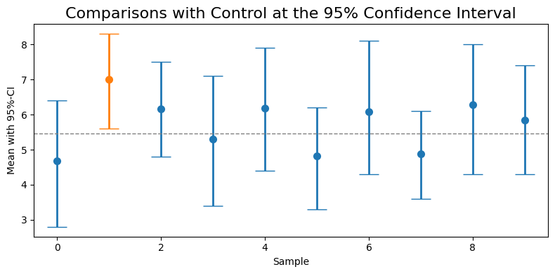
significant = [not (ci[0] <= mean_control <= ci[1]) for ci in ci_treatments]
colors = ['tab:blue' if not sig else 'tab:orange' for sig in significant]

# Plotting
fig, ax = plt.subplots(figsize=(8, 4))
for i, (mean, ci, color) in enumerate(zip(mean_treatments, ci_treatments, colors)):
    ax.scatter(i, mean, color=color, linewidth=2)
    ax.errorbar(i, mean, yerr=[[mean-ci[0]], [ci[1]-mean]], fmt='none', color=color, capsize=10, linewidth=2)

ax.axhline(mean_control, color='grey', linestyle='--', linewidth=1)
ax.set_xlabel("Sample")
ax.set_ylabel("Mean with 95%-CI")
ax.set_title('Comparisons with Control at the 95% Confidence Interval', fontsize=16)
plt.tight_layout()
plt.show()
data = np.array([1, 2, 3, 4, 5, 6, 7, 8, 9, 10])
mean = np.mean(data)
std_dev = np.std(data, ddof=1) # sample standard deviation
n = len(data)
sem = std_dev / np.sqrt(n)

# Manually compute the t-critical value for 95% CI and df = n - 1
# For df = 9, t_critical ≈ 2.262 (from standard t-distribution table)
t_critical = 2.262

margin_of_error = t_critical * sem
ci_lower = mean - margin_of_error
ci_upper = mean + margin_of_error

(ci_lower, ci_upper)
(3.3342998822551633, 7.665700117744837)
alpha = 0.05

bootstrap_means_control = bootstrap_mean(data, n_bootstrap=10, random_state=i)
bootstrap_means_treatment = bootstrap_mean(data_2, n_bootstrap=10, random_state=i)

boot_diffs = bootstrap_means_control - bootstrap_means_treatment
lower = np.percentile(boot_diffs, 100 * alpha / 2)
upper = np.percentile(boot_diffs, 100 * (1 - alpha / 2))
lower, upper
(-3.3550000000000004, -0.6366666666666667)
data = np.array([1, 2, 3, 4, 5, 6, 7, 8, 9, 10])
data_2 = np.array([5, 6, 7, 8, 9, 10])

bootstrap_means_control = bootstrap_mean(data, n_bootstrap=10, random_state=i)

for i in range(5):
    bootstrap_means_treatment = bootstrap_mean(data_2, n_bootstrap=10, random_state=i)
data = np.array([1, 2, 3, 4, 5, 6, 7, 8, 9, 10])
data_2 = np.array([5, 6, 7, 8, 9, 10])
results = {}
for i in range(5):
    bootstrap_means = bootstrap_mean(data_2, n_bootstrap=10, random_state=i)
    ci_lower, ci_upper = np.percentile(bootstrap_means, [2.5, 97.5])

    # bootstrap_mean = np.mean(bootstrap_means)
    # print(f"Bootstrap Mean Estimate: {bootstrap_mean:.2f}")
    print(f"Bootstrap Mean Estimate: {np.mean(bootstrap_means):.2f}")
    print(f"95% Confidence Interval: [{ci_lower:.2f}, {ci_upper:.2f}]")
    results[i] = {
        "mean": np.mean(bootstrap_means),
        "ci_lower": ci_lower,
        "ci_upper": ci_upper
    }
results
Bootstrap Mean Estimate: 7.55
95% Confidence Interval: [6.28, 8.76]
Bootstrap Mean Estimate: 7.38
95% Confidence Interval: [6.70, 7.96]
Bootstrap Mean Estimate: 7.67
95% Confidence Interval: [6.37, 8.96]
Bootstrap Mean Estimate: 7.28
95% Confidence Interval: [6.83, 8.00]
Bootstrap Mean Estimate: 7.93
95% Confidence Interval: [6.91, 9.39]
{0: {'mean': 7.549999999999999,
  'ci_lower': 6.279166666666667,
  'ci_upper': 8.758333333333335},
 1: {'mean': 7.383333333333333,
  'ci_lower': 6.704166666666667,
  'ci_upper': 7.9625},
 2: {'mean': 7.666666666666669,
  'ci_lower': 6.370833333333333,
  'ci_upper': 8.9625},
 3: {'mean': 7.283333333333333,
  'ci_lower': 6.833333333333333,
  'ci_upper': 8.0},
 4: {'mean': 7.9333333333333345,
  'ci_lower': 6.908333333333333,
  'ci_upper': 9.3875}}
Confidence Intervals#
Used to estimate a parameter, like the mean of a population.
From Supervised Machine Learning for Science [Freiesleben and Molnar, 2024]
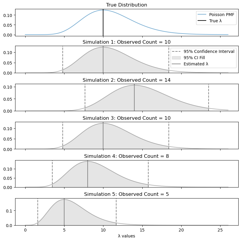
Frequentist confidence intervals represent the proportion of times we would see the true value of the parameter if we repeated the same experiment infinite times.
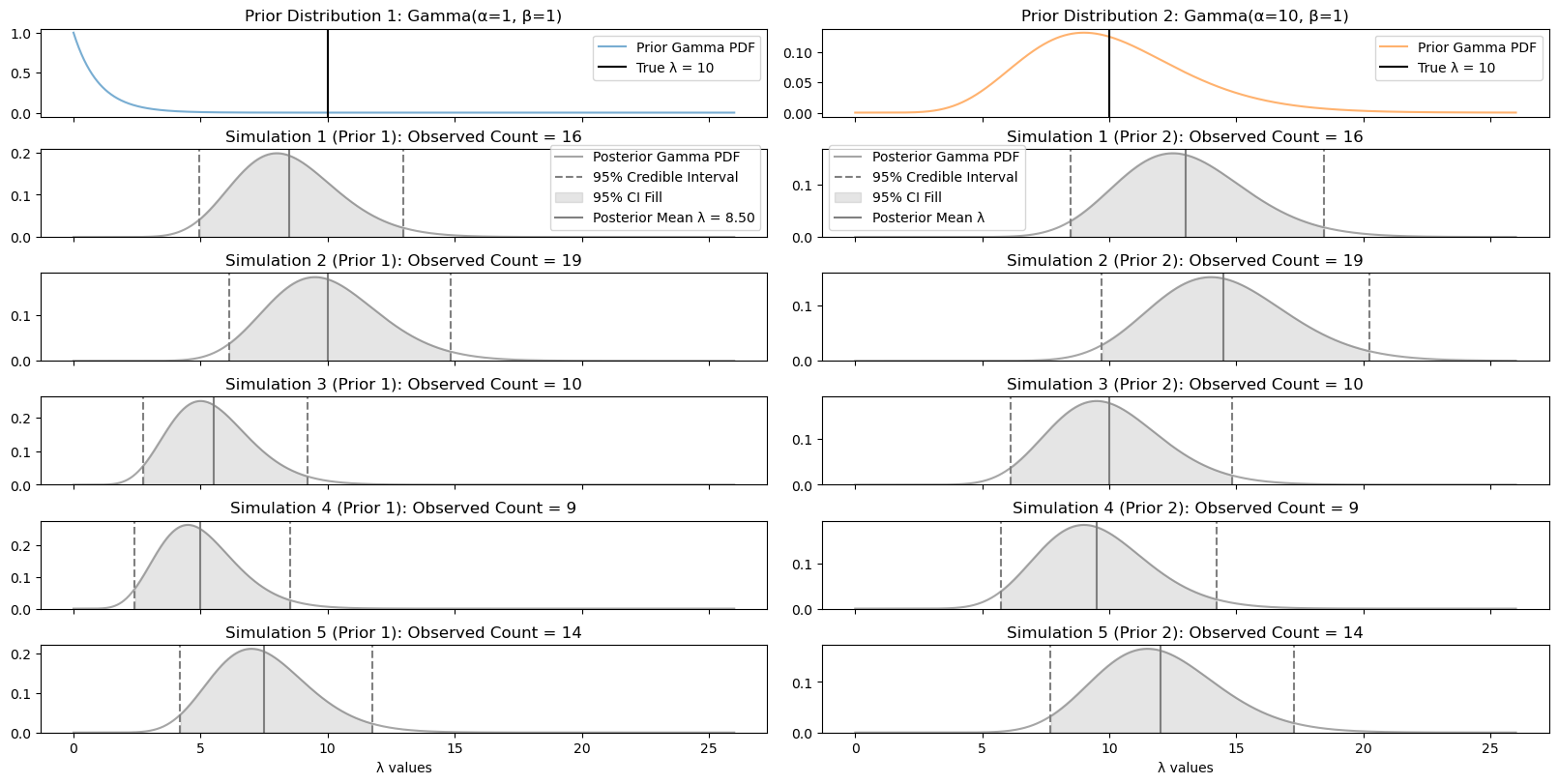
Bayesian credible intervals represent the probability that a distribution covers the true value. To construct a credible interval, we need a prior distribution.
Frequentist Confidence Intervals#
There are many ways to calculate CIs, here I use the Chi-Squared method to estimate a 95% confidence interval for the rate parameter (\(\lambda\)) of a Poisson distribution.
Show code cell source
import numpy as np
import scipy.stats as stats
import matplotlib.pyplot as plt

np.random.seed(42)
rng = np.random.default_rng(seed=42)

true_lambda = 10
n_simulations = 5

# Define a common range of λ values for all subplots
lambda_min = 0
lambda_max = true_lambda + 15
lambda_values = np.linspace(lambda_min, lambda_max + 1, 1000)
poisson_pmf = stats.poisson.pmf(true_lambda, lambda_values)

fig, axes = plt.subplots(n_simulations+1, 1, figsize=(8, 8), sharex=True, constrained_layout=True)
axes[0].plot(lambda_values, poisson_pmf, color='tab:blue', alpha=0.6, label='Poisson PMF')
axes[0].axvline(true_lambda, color='black', linestyle='-', label=f'True λ')
axes[0].set_title(f'True Distribution')
axes[0].legend()

for i in range(n_simulations):
    observed_count = rng.poisson(lam=true_lambda)
    estimated_lambda = observed_count

    # Construct a 95% confidence interval using the Chi-Squared method
    alpha = 0.05
    if observed_count == 0:
        lower_bound = 0
        upper_bound = 0.5 * stats.chi2.ppf(1 - alpha / 2, 2 * (observed_count + 1))
    else:
        lower_bound = 0.5 * stats.chi2.ppf(alpha / 2, 2 * observed_count)
        upper_bound = 0.5 * stats.chi2.ppf(1 - alpha / 2, 2 * (observed_count + 1))

    poisson_pmf = stats.poisson.pmf(observed_count, lambda_values)

    # Plot the Poisson PMF
    ax = axes[i+1]
    ax.plot(lambda_values, poisson_pmf, color='grey', alpha=0.6)
    ax.axvline(lower_bound, color='grey', linestyle='--', label='95% Confidence Interval' if i == 0 else "")
    ax.axvline(upper_bound, color='grey', linestyle='--')
    ax.fill_between(lambda_values, poisson_pmf,
                    where=(lambda_values >= lower_bound) & (lambda_values <= upper_bound),
                    color='grey', alpha=0.2, label='95% CI Fill' if i == 0 else "")
    ax.axvline(estimated_lambda, color='grey', linestyle='-', label=f'Estimated λ' if i == 0 else "")
    ax.set_title(f'Simulation {i+1}: Observed Count = {observed_count}')
    ax.set_ylim(0)
    # Display the legend only in the first subplot to avoid repetition
    if i == 0:
        ax.legend()

axes[-1].set_xlabel('λ values')
plt.show()
Baysian Credible Intervals#
There are multiple definitions for credible intervals. The most common:
Equal-Tailed Interval (ETI) / Quantile-Based Interval (QBI): This interval includes the cental \(1−\alpha\) proprotion of the posterior distribution. It is symmetrical about the tails. Often used when symmetry is desired and is more analogous to a frequentist confidence interval. It is what is used below.
Highest Density Interval (HDI): The HDI is the shortest interval that contains the specified probability mass \(1−\alpha\). Every point inside the HDI has a higher posterior density than any point outside the interval. It may not symmetrically exclude tails, especially for skewed distributions like the Gamma.
Show code cell source
alpha_prior_1 = 1
beta_prior_1 = 1

alpha_prior_2 = 10
beta_prior_2 = 1

fig, axes = plt.subplots(n_simulations + 1, 2, figsize=(16, 8), sharex=True, constrained_layout=True)

# Plot Prior Distribution for the first prior (Column 1)
prior_pdf_1 = stats.gamma.pdf(lambda_values, a=alpha_prior_1, scale=1/beta_prior_1)
axes[0, 0].plot(lambda_values, prior_pdf_1, color='tab:blue', alpha=0.6, label='Prior Gamma PDF')
axes[0, 0].axvline(true_lambda, color='black', linestyle='-', label=f'True λ = {true_lambda}')
axes[0, 0].set_title(f'Prior Distribution 1: Gamma(α={alpha_prior_1}, β={beta_prior_1})')
axes[0, 0].legend()

# Plot Prior Distribution for the second prior (Column 2)
prior_pdf_2 = stats.gamma.pdf(lambda_values, a=alpha_prior_2, scale=1/beta_prior_2)
axes[0, 1].plot(lambda_values, prior_pdf_2, color='tab:orange', alpha=0.6, label='Prior Gamma PDF')
axes[0, 1].axvline(true_lambda, color='black', linestyle='-', label=f'True λ = {true_lambda}')
axes[0, 1].set_title(f'Prior Distribution 2: Gamma(α={alpha_prior_2}, β={beta_prior_2})')
axes[0, 1].legend()


for i in range(n_simulations):
    observed_count = rng.poisson(lam=true_lambda)

    # --- Using Prior 1 ---
    # Update posterior parameters for Prior 1
    alpha_post_1 = alpha_prior_1 + observed_count
    beta_post_1 = beta_prior_1 + 1  # Assuming unit time interval or known exposure
    posterior_pdf_1 = stats.gamma.pdf(lambda_values, a=alpha_post_1, scale=1/beta_post_1)

    # Compute 95% Bayesian Credible Interval for Posterior 1
    lower_bound_1 = stats.gamma.ppf(0.025, a=alpha_post_1, scale=1/beta_post_1)
    upper_bound_1 = stats.gamma.ppf(0.975, a=alpha_post_1, scale=1/beta_post_1)
    posterior_mean_1 = alpha_post_1 / beta_post_1

    # Plot posterior distribution for Prior 1
    ax1 = axes[i + 1, 0]
    ax1.plot(lambda_values, posterior_pdf_1, color='grey', alpha=0.7, label='Posterior Gamma PDF')
    ax1.axvline(lower_bound_1, color='grey', linestyle='--', label='95% Credible Interval' if i == 0 else "")
    ax1.axvline(upper_bound_1, color='grey', linestyle='--')
    ax1.fill_between(lambda_values, posterior_pdf_1, where=(lambda_values >= lower_bound_1) & (lambda_values <= upper_bound_1),
                    color='grey', alpha=0.2, label='95% CI Fill' if i == 0 else "")
    ax1.axvline(posterior_mean_1, color='grey', linestyle='-', label=f'Posterior Mean λ = {posterior_mean_1:.2f}' if i == 0 else "")
    ax1.set_title(f'Simulation {i + 1} (Prior 1): Observed Count = {observed_count}')
    ax1.set_ylim(0)

    # Add legend only to the first posterior subplot in Column 1 to avoid repetition
    if i == 0:
        ax1.legend()

    # --- Using Prior 2 ---
    # Update posterior parameters for Prior 2
    alpha_post_2 = alpha_prior_2 + observed_count
    beta_post_2 = beta_prior_2 + 1  # Assuming unit time interval or known exposure
    posterior_pdf_2 = stats.gamma.pdf(lambda_values, a=alpha_post_2, scale=1/beta_post_2)

    # Compute 95% Bayesian Credible Interval for Posterior 2
    lower_bound_2 = stats.gamma.ppf(0.025, a=alpha_post_2, scale=1/beta_post_2)
    upper_bound_2 = stats.gamma.ppf(0.975, a=alpha_post_2, scale=1/beta_post_2)
    posterior_mean_2 = alpha_post_2 / beta_post_2

    # Plot posterior distribution for Prior 2
    ax2 = axes[i + 1, 1]
    ax2.plot(lambda_values, posterior_pdf_2, color='grey', alpha=0.7, label='Posterior Gamma PDF')
    ax2.axvline(lower_bound_2, color='grey', linestyle='--', label='95% Credible Interval' if i == 0 else "")
    ax2.axvline(upper_bound_2, color='grey', linestyle='--')
    ax2.fill_between(lambda_values, posterior_pdf_2, where=(lambda_values >= lower_bound_2) & (lambda_values <= upper_bound_2),
                    color='grey', alpha=0.2, label='95% CI Fill' if i == 0 else "")
    ax2.axvline(posterior_mean_2, color='grey', linestyle='-', label=f'Posterior Mean λ')
    ax2.set_title(f'Simulation {i + 1} (Prior 2): Observed Count = {observed_count}')
    ax2.set_ylim(0)

    # Add legend only to the first posterior subplot in Column 2 to avoid repetition
    if i == 0:
        ax2.legend()

# Label the x-axis on the bottom subplots for both columns
axes[-1, 0].set_xlabel('λ values')
axes[-1, 1].set_xlabel('λ values')
plt.show()
Timo Freiesleben and Christoph Molnar. Supervised Machine Learning for Science. Self-published, 2024. URL: https://ml-science-book.com/.