Optimization#
Network Flow#
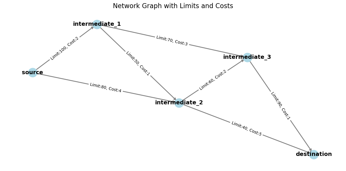
Optimize how to send goods from a source node to a destination node through a network while minimizing transportation costs. Each edge in the network has a capacity limit and a cost per unit flow. The goal is to determine the optimal flow through the network that meets demand at the destination without exceeding capacities.
import numpy as np
import pandas as pd
import cvxpy as cp
import matplotlib.pyplot as plt
import networkx as nx

nodes = ['source', 'intermediate_1', 'intermediate_2', 'intermediate_3', 'destination']
edges = [
    ('source', 'intermediate_1'),
    ('source', 'intermediate_2'),
    ('intermediate_1', 'intermediate_2'),
    ('intermediate_1', 'intermediate_3'),
    ('intermediate_2', 'intermediate_3'),
    ('intermediate_2', 'destination'),
    ('intermediate_3', 'destination'),
]
limits = {
    ('source', 'intermediate_1'): 100,
    ('source', 'intermediate_2'): 80,
    ('intermediate_1', 'intermediate_2'): 50,
    ('intermediate_1', 'intermediate_3'): 70,
    ('intermediate_2', 'intermediate_3'): 60,
    ('intermediate_2', 'destination'): 40,
    ('intermediate_3', 'destination'): 90,
}
costs = {
    ('source', 'intermediate_1'): 2,
    ('source', 'intermediate_2'): 4,
    ('intermediate_1', 'intermediate_2'): 1,
    ('intermediate_1', 'intermediate_3'): 3,
    ('intermediate_2', 'intermediate_3'): 2,
    ('intermediate_2', 'destination'): 5,
    ('intermediate_3', 'destination'): 1,
}

# Demand at each node (positive for demand, negative for supply)
demand = {
    'source': -100,  # Supply of 100 units
    'intermediate_1': 0,
    'intermediate_2': 0,
    'intermediate_3': 0,
    'destination': 100,   # Demand of 100 units
}

plt.figure(figsize=(12, 6))
G = nx.DiGraph()
G.add_nodes_from(nodes)

for edge in edges:
    G.add_edge(edge[0], edge[1])

pos = nx.spring_layout(G, seed=19)
nx.draw_networkx_nodes(G, pos, node_size=500, node_color='lightblue')
nx.draw_networkx_edges(G, pos, arrowstyle='->', arrowsize=12, edge_color='gray', width=2)
nx.draw_networkx_labels(G, pos, font_size=14, font_weight='bold')
edge_labels = {edge: f"Limit:{limits[edge]}, Cost:{costs[edge]}" for edge in edges}
nx.draw_networkx_edge_labels(G, pos, edge_labels=edge_labels, font_color='black', font_size=10)
plt.axis('off')
plt.title("Network Graph with Limits and Costs", fontsize=16)
plt.tight_layout()
plt.show()
# Create variables for flows on each edge
flow = {}
for edge in edges:
    flow[edge] = cp.Variable(nonneg=True)

# Objective: Minimize total transportation cost
total_cost = cp.sum([
    costs[edge] * flow[edge] for edge in edges
])
objective = cp.Minimize(total_cost)

constraints = []
for edge in edges:
    constraints.append(flow[edge] <= limits[edge])

# Flow conservation at each node
for node in nodes:
    inflow = cp.sum([
        flow[(i, j)] for (i, j) in edges if j == node
    ])
    outflow = cp.sum([
        flow[(i, j)] for (i, j) in edges if i == node
    ])
    # Net flow equals demand
    constraints.append(inflow - outflow == demand.get(node, 0))

# Solve the problem
problem = cp.Problem(objective, constraints)
problem.solve()

print(f"Minimum total transportation cost: ${problem.value:.2f}\n")
print("Optimal flow on each edge:")
for edge in edges:
    flow_value = flow[edge].value if flow[edge].value is not None else 0
    print(f"Flow from {edge[0]} to {edge[1]}: {flow_value:.2f} units")
Minimum total transportation cost: $620.00

Optimal flow on each edge:
Flow from source to intermediate_1: 100.00 units
Flow from source to intermediate_2: 0.00 units
Flow from intermediate_1 to intermediate_2: 41.43 units
Flow from intermediate_1 to intermediate_3: 58.57 units
Flow from intermediate_2 to intermediate_3: 31.43 units
Flow from intermediate_2 to destination: 10.00 units
Flow from intermediate_3 to destination: 90.00 units
Portfolio Optimization#
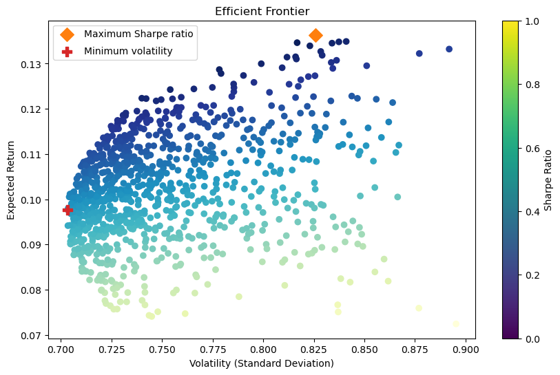
Portfolio optimization has two competing objectives: high return and low risk.
Variables:
\(\mu\): Expected returns
\(N\): Number of assets
\(w_i\): Fraction of money to invest in asset \(i\)
\(\Sigma\): Covariance matrix which quantifies how different assets in a portfolio move relative to each other.
\(\gamma>0\): Risk aversion parameter
Objective: maximize \(\mu^T w - \gamma w^T\Sigma w\) (risk-adjusted return)
Constraints:
\(\sum_{i=0}^N w_i = 1\)
\(w_i >= 0\)
expected_returns = np.array([0.08, 0.12, 0.15, 0.06])  # [Bonds, VTI, International, Small-Cap]
weights = cp.Variable(len(expected_returns))
risk_aversion = 0.0

covariance_matrix = np.array([
    [1.0, 0.3, 0.2, 0.1],
    [0.3, 1.0, 0.4, 0.5],
    [0.2, 0.4, 1.0, 0.6],
    [0.1, 0.5, 0.6, 1.0]
])

constraints = [cp.sum(weights) == 1, weights >= 0]
portfolio_variance = cp.quad_form(weights, covariance_matrix)
objective = cp.Maximize(expected_returns.T @ weights - portfolio_variance * risk_aversion)
problem = cp.Problem(objective, constraints)
problem.solve()
optimal_weights = weights.value
optimal_weights
array([-2.14111410e-28, -2.14377958e-28, 1.00000000e+00, -2.13978135e-28])
def calculate_portfolio_performance(weights, expected_returns, covariance_matrix):
    portfolio_return = np.dot(weights, expected_returns)
    portfolio_risk = np.sqrt(np.dot(weights.T, np.dot(covariance_matrix, weights)))
    return portfolio_return, portfolio_risk

risk_free_rate = 0.03
num_portfolios = 1000
results = np.zeros((3, num_portfolios))
weights_record = []

for i in range(num_portfolios):
    weights = np.random.random(len(expected_returns))
    weights /= np.sum(weights)
    portfolio_return, portfolio_risk = calculate_portfolio_performance(weights, expected_returns, covariance_matrix)
    results[0,i] = portfolio_risk
    results[1,i] = portfolio_return
    results[2,i] = (portfolio_return - risk_free_rate) / portfolio_risk  # Sharpe ratio
    weights_record.append(weights)

max_sharpe_idx = np.argmax(results[2])
sdp, rp = results[0, max_sharpe_idx], results[1, max_sharpe_idx]
max_sharpe_allocation = pd.DataFrame(weights_record[max_sharpe_idx], index=['Bonds', 'VTI', 'International', 'Small-Cap'], columns=['allocation'])

min_vol_idx = np.argmin(results[0])
sdp_min, rp_min = results[0, min_vol_idx], results[1, min_vol_idx]
min_vol_allocation = pd.DataFrame(weights_record[min_vol_idx], index=['Bonds', 'VTI', 'International', 'Small-Cap'], columns=['allocation'])

plt.figure(figsize=(10, 6))
plt.scatter(results[0, :], results[1, :], c=results[2, :], cmap='YlGnBu', marker='o')
plt.scatter(sdp, rp, marker='D', color='tab:orange', s=100, label='Maximum Sharpe ratio')
plt.scatter(sdp_min, rp_min, marker='P', color='tab:red', s=100, label='Minimum volatility')

plt.title('Efficient Frontier')
plt.xlabel('Volatility (Standard Deviation)')
plt.ylabel('Expected Return')
plt.colorbar(label='Sharpe Ratio')
plt.legend(labelspacing=0.8)
plt.show()