Statistical Tests (A/B Testing)

Statistical Tests (A/B Testing)#

Steps to Assess Statistical Significance: #

Formulate Hypotheses:
- Null Hypothesis (\(H_0\)): There is no effect, and any observed results are due to random chance.
- Alternative Hypothesis (\(H_a\)): There is a real effect or difference.
Choose Significance Level (\(α\)): The probability of rejecting the null hypothesis when it is true (Type I error). Commonly 0.05.
Select Statistical Test: Common tests include t-tests, chi-square tests, ANOVA, and regression analysis.
Calculate Test Statistic and P-value.

Note: In a business context, it’s also important to clarify the purpose and value of the experiment. Is it worth running a test? Define metrics:

Success metrics that quantify a desired change.
Tracking metrics help explain the movement in the success metrics.
Guardrail metrics that you do not want to harm.

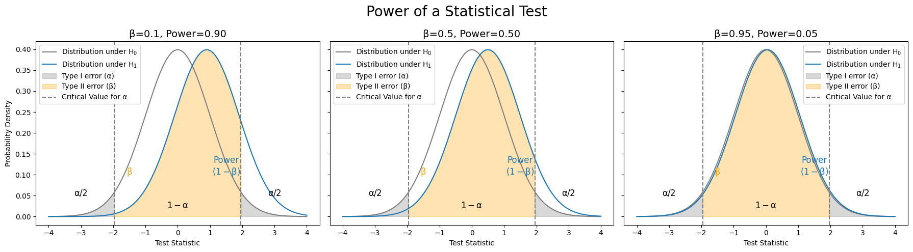
Sample Size and Statistical Power:
#

	\(H_0\) is True	\(H_0\) is False
Test Rejects \(H_0\)	Significance Level (\(α\))	Power (\(1-β\))
Test Accepts \(H_0\)	\(1-α\)	\(β\)

Where

\(α\) = probability of a Type I error, known as a “false positive”.
\(β\) = probability of a Type II error, known as a “false negative”.
\(1 − α\) = probability of a “true negative”, i.e., correctly not rejecting the null hypothesis.
\(1 − β\) = probability of a “true positive”, i.e., correctly rejecting the null hypothesis. The power of the test.

../_images/0f3379ec26a4c9b61be86c5d239b4c8c9e6420abe7edfb3b55c76046d2d74089.png

Note

The alpha and p-value are not the same!

Alpha (\(\alpha\)): The pre-determined probability of incorrectly rejecting a null hypothesis that is actually true.
P-value: The probability of getting a result at least as extreme as observed in the sample. It’s computed from the sample data, based on the type of test.

If \( \text{p-value} < \alpha \) then the null hypothesis is rejected.

“the probability that the data could have arisen if the null hypothesis is true,” is not the same as, “the probability that the null hypothesis is true given the data.” [Cohen, 1994]

Sample Size and Minimum Detectable Effect#

Handy calculators are available online for this such as [Kohn and Senyak, 2025]

p0 = 0.1  # Baseline conversion rate
p1 = 0.2  # Target conversion rate
alpha = 0.05  # Significance level
power = .8  # Power

# Z-scores for significance level and power
z_alpha = stats.norm.ppf(1 - alpha / 2)  # Two-tailed test
z_beta = stats.norm.ppf(power)

# Variance for baseline and target rates
var_p0 = p0 * (1 - p0)
var_p1 = p1 * (1 - p1)
pooled_proportion = p0 * (1 - p0) + p1 * (1 - p1)

# Minimum Detectable Effect (MDE)
mde = p1 - p0

# Sample size formula
n = ((z_alpha + z_beta) ** 2 * (var_p0 + var_p1)) / (mde ** 2)
sample_size = np.ceil(n)  # Round up to the nearest whole number

print(f"Required sample size per group: {sample_size}")
print(f"Total required sample size: {sample_size * 2}")

Required sample size per group: 197.0
Total required sample size: 394.0

print(f'The standard normal deviate for α = Zα = {z_alpha:.4f}')
print(f'The standard normal deviate for β = Zβ = {z_beta:.4f}')

The standard normal deviate for α = Zα = 1.9600
The standard normal deviate for β = Zβ = 0.8416

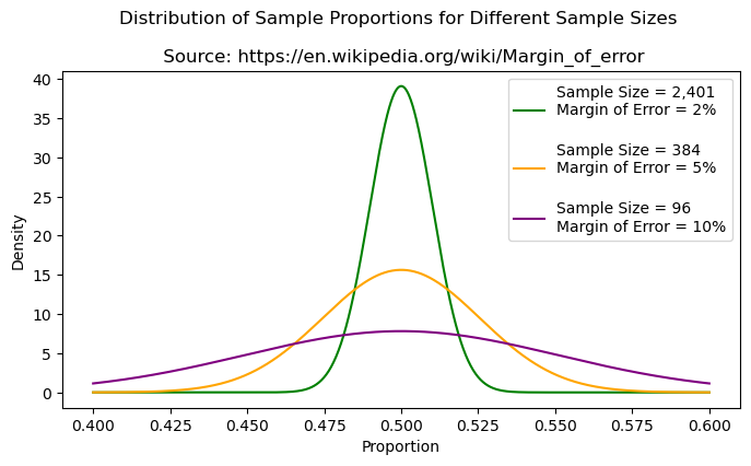
Margin of Error (MoE) #

Expresses the sampling error in a survey’s results. It is a range within which the true population parameter is expected to lie, with a certain level of confidence. Used for many things including sample size determination.

Sample Proportion MoE#

\[\text{MoE} = z \times \sqrt{\frac{p(1-p)}{n}}\]

Where:

z is the critical value from the standard normal distribution corresponding to the desired confidence level (e.g., 1.96 for 95% confidence).
p is the sample proportion.
n is the sample size.

Sample Mean MoE#

\[ \text{MoE} = t \times \frac{s}{\sqrt{n}} \]

Where:

t is the critical value from the t-distribution corresponding to the desired confidence level and degrees of freedom.
s is the sample standard deviation.
n is the sample size.

../_images/5ddd2e38941b5263dd05be18d648a52d08a5d15799e76c8a38d7e75f257e7286.png

Confidence Intervals (CI) #

CI is a range of values that are likely to contain the true population parameter (e.g. mean) with a level of confidence. The confidence level represents the proportion of times that the CI would contain the true parameter if the same population were sampled multiple times.

Misrepresentation: “There is a 95% probability that the true parameter lies within this interval.”
True Interpretation: “If we were to take many samples and construct a confidence interval from each sample, we expect 95% of those intervals to contain the true parameter. For any given interval, the true parameter either is in the interval or it isn’t.”

Great overview on the topic: Confidence Intervals by Lisa Sullivan, PhD

Confidence Interval for One Sample:

\[ \text{One Sample Confidence Interval} = \text{Sample Mean} \pm MoE \]

Example: Estimate the average test score of students in a school based on a random sample.

sample_size = 50
sample_mean = 80
sample_std_dev = 20
z = 1.96  # Z value for 95% confidence is 1.96
MoE = z * sample_std_dev / sample_size

print(f"Confidence interval: ({sample_mean - MoE:0.2f}, {sample_mean + MoE:0.2f})")
print(f"Interpretation: we are 95% confident that the true mean is between {sample_mean - MoE:0.2f} and {sample_mean + MoE:0.2f}.")

Confidence interval: (79.22, 80.78)
Interpretation: we are 95% confident that the true mean is between 79.22 and 80.78.

Confidence Interval for Two Independent Samples:

\[ \text{Standard Error (SE)} = \sqrt{\frac{s^2_1}{n_1} + \frac{s^2_2}{n_2}} \]

\[ \text{Margin of Error (MoE)} = z * SE \]

\[ \text{Two Sample Confidence Interval} = \bar{x_1} - \bar{x_2} \pm MoE \]

Example: Compare the average test scores of students from two different schools.

mean_1 = 100
mean_2 = 85
std_dev_1 = 15
std_dev_2 = 20
sample_size_1 = 30
sample_size_2 = 25
z = 1.96  # Z value for 95% confidence
standard_error = ((std_dev_1**2 / sample_size_1) + \
                  (std_dev_2**2 / sample_size_2))**0.5
MoE = z * standard_error
mean_diff = mean_1 - mean_2
print(f"Confidence interval: ({mean_diff - MoE:0.2f}, {mean_diff + MoE:0.2f})")
print(f"Interpretation: We are 95% confident that the true difference between the population means lies between {mean_diff - MoE:0.2f} and {mean_diff + MoE:0.2f}.")

Confidence interval: (5.50, 24.50)
Interpretation: We are 95% confident that the true difference between the population means lies between 5.50 and 24.50.

Common Statstical Tests #

Z-tests / T-tests: Compare the means of two groups.#

When to use a Z-test vs. T-test?: Generally, Z-Tests are used when the sample size (\(n\)) is less than 30.
Assumptions: Normal distribution of data, equal variances between groups, and independence of observations.
Types:
- One-sample T-Test: Compares the means of the sample data to the population (e.g., Sample from a factory process).
- Independent (Two-sample) T-test: Compares the means of two independent groups (e.g., comparing the heights of men and women).
– Welch’s T-Test for Unequal Variances should be used instead of the independent t-test regardless since it is more robust. It can be applied without any substantial disadvantages to Student’s t-test. It’s not recommended to pre-test for equal variances and then choose between Student’s t-test or Welch’s t-test.
- Dependent (Paired) T-test: Compares the means of two related groups (e.g., comparing the weights of individuals before and after a diet).

ANOVA (Analysis of Variance): Compare the means of three or more groups.#

Assumptions: Assumes normal distribution of data, homogeneity of variances, and independence of observations.
Types:
- One-way ANOVA: Compares the means of multiple groups based on one factor (e.g., comparing the test scores of students from different schools).
- Two-way ANOVA: Compares the means of groups based on two factors (e.g., comparing the test scores of students from different schools and different grades).

Note

A one way ANOVA with two independent groups is mathematically equivalent to an independent t-test. In the two-group case, the F-statistic from ANOVA is just the square of the t-statistic from the t-test:

\[ F = t^2 \]

Wilcoxon Signed-Rank Test: Non-parametric test to compare the median of a set of numbers against a hypothetical median.#

Assumptions: The data should be ordinal, interval, or ratio scales where ranking is meaningful. While it does not require normality, it assumes that the differences between pairs are symmetrically distributed around the median.
Note: More robust alternative to the t-test when dealing with outliers, as it is less sensitive to extreme values due to its reliance on ranks rather than raw data.

The Wilcoxon signed-ranks test is the nonparametric alternative for the dependent t-test.

Mann-Whitney U-Test: Non-parametric test to determine whether a numeric outcome variable with any distribution differs across two independent groups.#

Assumptions: The data should be ordinal, interval, or ratio scales where ranking is meaningful. While it does not require normality, it assumes that the differences between pairs are symmetrically distributed around the median.
Note: This test does not test specifically if the mean or median of two groups are equal, only if the overall distributions are significantly different or not [Mann-Whitney U-Test, n.d.].

The Mann-Whitney U is the nonparametric alternative to the independent t-test.

Chi-squared Tests: Test the relationship between categorical variables.#

Assumptions: Assumes a sufficient sample size (expected frequencies in each cell should be at least 5) and independence of observations.
Types:
- Independence: Assesses whether there is an association between two categorical variables (e.g., gender and voting preference).
- Goodness-of-Fit: Tests whether the distribution of a single categorical variable matches an expected distribution (e.g., testing if a die is fair).
- Homogeneity: Test if samples came from the same population.

Fisher’s Exact Test: Test relationship between categorical variables for small sample sizes or small expected frequencies Assumptions: Assumes a sufficient sample size (expected frequencies in each cell should be at least 5) and independence of observations.

G-test (Likelihood Ratio Test): Increasingly being used over chi-squared tests due to better accuracy and interpretability in some cases, but note that it is unreliable if the sample sizes are small.

Examples#

T-Tests: One-Sample#

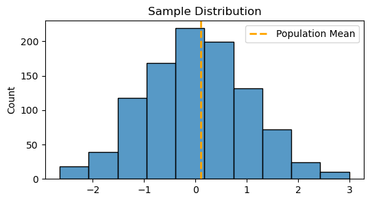
When you need to compare the mean from a single sample against a known or hypothesized population mean under assumptions of normality and random sampling.

import pandas as pd
import seaborn as sns
import warnings
warnings.simplefilter(action='ignore', category=FutureWarning)

rng = np.random.default_rng()

data = rng.standard_normal(1000)
pop_mean = 0.1 # Known or hypothesized population mean
t_stat, p_value = stats.ttest_1samp(data, pop_mean)

print(f"T-statistic: {t_stat:.04f}")
print(f"P-value: {p_value:.04f}")
if p_value > 1-0.05:  # 5% significance level
    print("Reject the null hypothesis - sample mean is significantly different from the population mean.")
else:
    print("Fail to reject the null hypothesis - sample mean is not significantly different from the population mean.")

plt.figure(figsize=(6, 3))
sns.histplot(data, bins=10, color='#1f77b4')
plt.axvline(x=pop_mean, color='orange', linestyle='--', linewidth=2, label='Population Mean')
plt.title('Sample Distribution')
plt.legend()
plt.show()

T-statistic: -2.4978
P-value: 0.0127
Fail to reject the null hypothesis - sample mean is not significantly different from the population mean.

../_images/2cae058128589eb370a59e59bd9396ec29042fa70f44fd0d3b4d1a7b8d933516.png

T-Tests: Independent (Two-sample)#

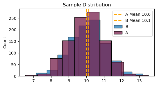
Groups: Compares the means of two independent groups. Subjects in one group have no connection to the subjects in the other group.
Examples: Comparing the heights of men and women, or test scores of students from two different schools

A = rng.normal(10, 1, 1000)
B = rng.normal(10.1, 1, 1000)

t_stat, p_value = stats.ttest_ind(A, B, equal_var=True)
print(f"T-Test Assuming Equal Variance:")
print(f"\tT-statistic: {t_stat:.04f}")
print(f"\tP-value: {p_value:.04f}")

t_stat, p_value = stats.ttest_ind(A, B, equal_var=False)
print(f"\nWelch's T-Test for Unequal Variance:")
print(f"\tT-statistic: {t_stat:.04f}")
print(f"\tP-value: {p_value:.04f}")

plt.figure(figsize=(6, 3))
sns.histplot(B, bins=10, color='#1f77b4', label='B')
sns.histplot(A, bins=10, color='#771f4b', label='A')
plt.axvline(x=A.mean(), color='orange', linestyle='--', linewidth=2, label=f'A Mean {A.mean():.01f}')
plt.axvline(x=B.mean(), color='orange', linestyle='--', linewidth=2, label=f'B Mean {B.mean():.01f}')
plt.title('Sample Distribution')
plt.legend()
plt.show()

T-Test Assuming Equal Variance:
	T-statistic: -2.1062
	P-value: 0.0353

Welch's T-Test for Unequal Variance:
	T-statistic: -2.1062
	P-value: 0.0353

../_images/8091a83e5104fa665764889713d4bc6eb1615453080255c7a0830333750eb95a.png

Welch’s t-test for unequal variance#

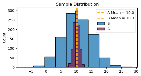
A = rng.normal(10, 1, 1000)
B = rng.normal(10.4, 5, 1000)

t_stat, p_value = stats.ttest_ind(A, B, equal_var=True)
print(f"T-Test Assuming Equal Variance:")
print(f"\tT-statistic: {t_stat:.04f}")
print(f"\tP-value: {p_value:.04f}")

t_stat, p_value = stats.ttest_ind(A, B, equal_var=False)
print(f"\nWelch's T-Test for Unequal Variance:")
print(f"\tT-statistic: {t_stat:.04f}")
print(f"\tP-value: {p_value:.04f}")

plt.figure(figsize=(6, 3))
sns.histplot(B, bins=10, color='#1f77b4', label='B')
sns.histplot(A, bins=10, color='#771f4b', label='A')
plt.axvline(x=A.mean(), color='orange', linestyle='--', linewidth=2, label=f'A Mean = {A.mean():.01f}')
plt.axvline(x=B.mean(), color='orange', linestyle='--', linewidth=2, label=f'B Mean = {B.mean():.01f}')
plt.title('Sample Distribution')
plt.legend()
plt.show()

T-Test Assuming Equal Variance:
	T-statistic: -1.8134
	P-value: 0.0699

Welch's T-Test for Unequal Variance:
	T-statistic: -1.8134
	P-value: 0.0700

../_images/d4bb4c17875fa50fb098f211a720531087e1303ed17abb42920f0103d8c1a34d.png

T-Tests: Paired (Dependent)#

Groups: Compares the means of two related groups. Subjects in these groups are connected. Typically through repeated measurements on the same subjects.
Examples: Comparing the weights of individuals before and after a diet, or the test scores of students before and after a specific training program

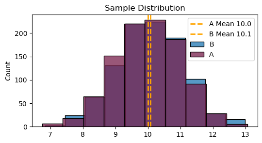
A = rng.normal(10, 1, 1000)
B = rng.normal(10.1, 1, 1000)

t_stat, p_value = stats.ttest_ind(A, B, equal_var=True)
print(f"Independent T-Test:")
print(f"\tT-statistic: {t_stat:.04f}")
print(f"\tP-value: {p_value:.04f}")


t_stat, p_value = stats.ttest_rel(A, B) # Before and After
print(f"\nPaired T-Test:")
print(f"\tT-statistic: {t_stat:.04f}")
print(f"\tP-value: {p_value:.04f}")

plt.figure(figsize=(6, 3))
sns.histplot(B, bins=10, color='#1f77b4', label='B')
sns.histplot(A, bins=10, color='#771f4b', label='A')
plt.axvline(x=A.mean(), color='orange', linestyle='--', linewidth=2, label=f'A Mean {A.mean():.01f}')
plt.axvline(x=B.mean(), color='orange', linestyle='--', linewidth=2, label=f'B Mean {B.mean():.01f}')
plt.title('Sample Distribution')
plt.legend()
plt.show()

Independent T-Test:
	T-statistic: -1.7186
	P-value: 0.0858

Paired T-Test:
	T-statistic: -1.7073
	P-value: 0.0881

../_images/a4a09c514a9ead3f8b95468822d5d50e89d4859090bcb5e707aea4767df5178c.png

Wilcoxon Signed-Rank Test#

# Data: Sleep duration in hours for 10 participants
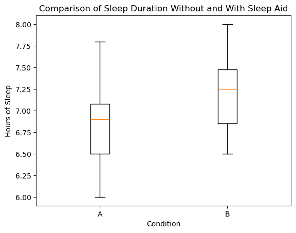
A = np.array([7, 6.5, 7.2, 6, 7.8, 6.5, 7, 6.8, 7.1, 6.3]) # Group A: Without sleep aid
B = np.array([7.5, 6.8, 7.4, 6.5, 8, 7, 7.5, 7.2, 7.3, 6.8]) # Group B: With sleep aid
stat, p_value = stats.wilcoxon(A - B)
print(f"Test Statistic: {stat:.04}")
print(f"P-Value: {p_value:.04f}")

if p_value < 0.05:
    print("Reject the null hypothesis - suggest a significant difference in sleep duration.")
else:
    print("Fail to reject the null hypothesis - no significant difference in sleep duration.")

t_stat, p_value = stats.ttest_ind(A, B)
print("\nIndependent T-Test on the same data:")
print(f"\tTest Statistic: {stat:.04}")
print(f"\tP-Value: {p_value:.04f}")

t_stat, p_value = stats.ttest_rel(A, B)
print("\nPaired T-Test on the same data:")
print(f"\tTest Statistic: {stat:.04}")
print(f"\tP-Value: {p_value:.05f}")

fig, ax = plt.subplots()
ax.boxplot([A, B], labels=['A', 'B'])
ax.set_title('Comparison of Sleep Duration Without and With Sleep Aid')
ax.set_ylabel('Hours of Sleep')
ax.set_xlabel('Condition')
plt.show()

Test Statistic: 0.0
P-Value: 0.0020
Reject the null hypothesis - suggest a significant difference in sleep duration.

Independent T-Test on the same data:
	Test Statistic: 0.0
	P-Value: 0.0925

Paired T-Test on the same data:
	Test Statistic: 0.0
	P-Value: 0.00001

../_images/75309fab56d7026cca702dec878462a06278c6899c1e86f75ccc38cf156f504f.png

Chi-square Goodness of Fit#

Note that chi2_contingency performs a two-sided test, so we’re checking for positve and negative effects.

Khan Academy: Contingency table chi-square test

Null Hypothesis: Herbs do nothing
Alternative Hypothesis: Herbs do something

#                 Herb 1      Herb 2   Placebo
data = np.array([[20,         30,      30],        # Sick 
                 [100,        110,     90]])       # Not Sick

chi2_stat, p_value, dof, expected = stats.chi2_contingency(data)
print(f"Chi-squared Statistic: {chi2_stat:.04f}")
print(f"P-value: {p_value:.04f}")

Chi-squared Statistic: 2.5258
P-value: 0.2828

Chi-squared Independence / Fisher’s Exact Test / G-Test#

# Rows represent categories of variable 1 (e.g., Gender: Male, Female)
# Columns represent categories of variable 2 (e.g., Preference: Yes, No)
contingency_table = np.array([[30, 20],   #   Male: 30 Yes, 20 No
                              [35, 15]])  # Female: 35 Yes, 15 No

chi2_stat, p_val, dof, expected = stats.chi2_contingency(contingency_table)
print(f"Chi-squared statistic: {chi2_stat:.02f}")
print(f"P-value: {p_val:.04f}\n")

odds_ratio, p_value = stats.fisher_exact(contingency_table)
print(f"Fisher's Exact Test statistic: {odds_ratio:.04f}")
print(f"P-value: {p_value:.04f}\n")

chi2_stat, p_val, dof, expected = stats.chi2_contingency(contingency_table, lambda_="log-likelihood")
print(f"G-Test statistic: {chi2_stat:.02f}")
print(f"P-value: {p_val:.04f}\n")

Chi-squared statistic: 0.70
P-value: 0.4017

Fisher's Exact Test statistic: 0.6429
P-value: 0.4019

G-Test statistic: 0.70
P-value: 0.4013

""" Source: Berger, Jeffrey S. et al. “Aspirin for the Primary Prevention of Cardiovascular Events in Women and Men: A Sex-Specific Meta-analysis of Randomized Controlled Trials.” JAMA, 295(3):306-313, DOI:10.1001/jama.295.3.306, 2006.
        https://jamanetwork.com/journals/jama/article-abstract/202217
        
                    Aspirin   Control/Placebo
Ischemic stroke       176           230
No stroke           21035         21018
"""
contingency_table = np.array([[176, 230], 
                              [21035, 21018]])

chi2_stat, p_val, dof, expected = stats.chi2_contingency(contingency_table)
print(f"Chi-squared statistic: {chi2_stat:.02f}")
print(f"P-value: {p_val:.04f}\n")

odds_ratio, p_value = stats.fisher_exact(contingency_table)
print(f"Fisher's Exact Test statistic: {odds_ratio:.04f}")
print(f"P-value: {p_value:.04f}\n")

chi2_stat, p_val, dof, expected = stats.chi2_contingency(contingency_table, lambda_="log-likelihood")
print(f"G-Test statistic: {chi2_stat:.02f}")
print(f"P-value: {p_val:.04f}\n")

Chi-squared statistic: 6.89
P-value: 0.0087

Fisher's Exact Test statistic: 0.7646
P-value: 0.0081

G-Test statistic: 6.91
P-value: 0.0086

Chi-square Goodness-of-Fit Test:#

Khan Academy Example

#          Day:     M   T   W   T   F   S
expected_freq =   [.1, .1, .15, .2, .3, .15]  # Expected frequencies in each category. By default the categories are assumed to be equally likely.
observed_counts = [30, 14, 34, 45, 57, 20]  # Observed values in each category.
observed_freq = [i/sum(observed_counts) for i in observed_counts] # Normalize observed values to frequencies.
expected_counts = [int(i*sum(observed_counts)) for i in expected_freq]

chi2_stat, p_value = stats.chisquare(f_obs=observed_counts, f_exp=expected_counts)

print(f"Chi-squared Statistic: {chi2_stat:.04f}")
print(f"P-value: {p_value:.04f}")

Chi-squared Statistic: 11.4417
P-value: 0.0433

G-Test (Goodness-of-Fit):#

observed_counts = np.array(observed_counts)
expected_counts = np.array(expected_counts)
G_statistic = 2 * np.sum(observed_counts * np.log(observed_counts / expected_counts))
degrees_of_freedom = len(observed_counts) - 1
p_value = stats.chi2.sf(G_statistic, degrees_of_freedom)
print(f"G-statistic: {G_statistic:.04f}")
print(f"P-value: {p_value:.04f}")

G-statistic: 11.3865
P-value: 0.0442

One-way ANOVA#

Tests whether two or more groups have the same population mean.

Zedstatstics Example

\( \text{Sum of Squares = SST} = \sum ({X - \overline{X}})^2 \)

\( \text{Sum of Squares Within Groups = SSW} = \sum ({\overline{X} - \overline{\overline{X}_i}})^2 \)

\( \text{Sum of Squares Between Groups = SSB} = \sum ({X_i - \overline{X}})^2 \)

\( \text{F} = \frac{\frac{\text{SSB}}{c - 1}} {\frac{\text{SSW}}{n - c}} \\ \text{Where:} \\ \quad \text{c = number of categories} \\ \quad \text{n = number of observations} \)

def SSW(group):
    X_bar = sum(group) / len(group)
    return sum([(num-X_bar)**2 for num in group])

def SSB(group, global_mean):
    X_bar = sum(group) / len(group)
    return len(group) * (X_bar - global_mean)**2

def f_stat(SSB, SSW, n, c):
    return (SSB / (c-1)) / ((SSW)/(n-c))

group1 = [1, 5, 9]
group2 = [3, 5, 7]
group3 = [4, 5, 6]
groups = [group1, group2, group3]

n = sum([len(group) for group in groups])
c = len(groups)
group_means = [sum(group)/len(group) for group in groups]
global_mean = sum(group_means) / len(group_means)

for group in groups:
    print(group, "     F-Statstic:", f_stat(SSB(group, global_mean), SSW(group), n, c), "   SSW:", SSW(group), "   SSB:", SSB(group, global_mean))

[1, 5, 9]      F-Statstic: 0.0    SSW: 32.0    SSB: 0.0
[3, 5, 7]      F-Statstic: 0.0    SSW: 8.0    SSB: 0.0
[4, 5, 6]      F-Statstic: 0.0    SSW: 2.0    SSB: 0.0

group1 = [1, 3, 5]
group2 = [5, 7, 9]
group3 = [4, 5, 6]
groups = [group1, group2, group3]

n = sum([len(group) for group in groups])
c = len(groups)
group_means = [sum(group)/len(group) for group in groups]
global_mean = sum(group_means) / len(group_means)

for group in groups:
    print(group, "     F-Statstic:", f_stat(SSB(group, global_mean), SSW(group), n, c), "   SSW:", SSW(group), "   SSB:", SSB(group, global_mean))

[1, 3, 5]      F-Statstic: 4.5    SSW: 8.0    SSB: 12.0
[5, 7, 9]      F-Statstic: 4.5    SSW: 8.0    SSB: 12.0
[4, 5, 6]      F-Statstic: 0.0    SSW: 2.0    SSB: 0.0

group1 = [20, 21, 19, 22, 24]
group2 = [28, 32, 30, 29, 27]
group3 = [25, 29, 27, 26, 28]
f_statistic, p_value = stats.f_oneway(group1, group2, group3) # Perform one-way ANOVA
print(f"F-statistic: {f_statistic:.04f}")
print(f"P-value: {p_value:.06f}")

F-statistic: 25.8788
P-value: 0.000044

Permutation Test#

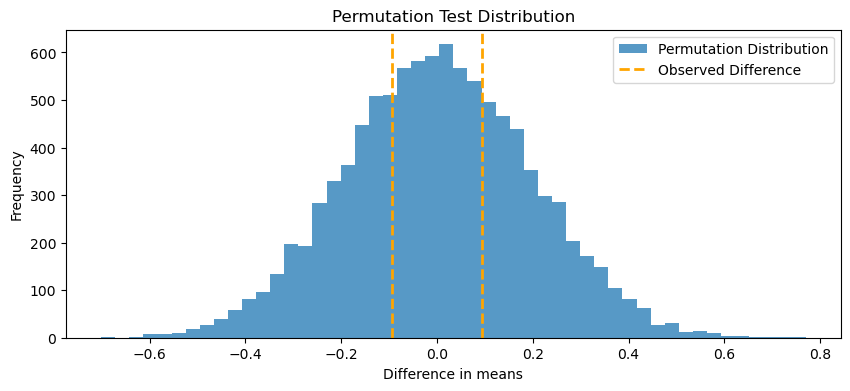
A non-parametric method used to assess the statistical significance by evaluating all possible rearrangements of the data under the null hypothesis.

Steps:

Compute the test statistic (e.g., difference in means) for the observed data.
Randomly shuffle the labels or group assignments of the data points.
Recalculate the test statistic for each shuffled dataset.
Repeat the shuffling process many times to build a distribution of the test statistic under the null hypothesis.
Determine the p-value by assessing where the original test statistic falls within this distribution.

def perform_permutation_test(combined, size1, size2, num_permutations=10000):
    perm_diffs = np.zeros(num_permutations)
    for i in range(num_permutations):
        np.random.shuffle(combined)
        new_group1 = combined[:size1]
        new_group2 = combined[size1:size1+size2]
        perm_diffs[i] = np.mean(new_group2) - np.mean(new_group1)
    return perm_diffs

data_group1 = rng.standard_normal(sample_size)  # Mean score group 1
data_group2 = rng.standard_normal(sample_size) # Mean score of group 2
observed_diff = np.mean(data_group2) - np.mean(data_group1)
combined_data = np.concatenate([data_group1, data_group2])

# Perform the permutation test
perm_diffs = perform_permutation_test(combined_data.copy(), len(data_group1), len(data_group2))
p_value = np.mean(np.abs(perm_diffs) >= np.abs(observed_diff))
print(f"Observed difference in means: {observed_diff:.04f}")
print(f"P-value from permutation test: {p_value:.04f}")

plt.figure(figsize=(10,4))
plt.hist(perm_diffs, bins=50, alpha=0.75, label='Permutation Distribution')
plt.axvline(x=observed_diff, color='orange', linestyle='dashed', linewidth=2, label='Observed Difference')
plt.axvline(x=-observed_diff, color='orange', linestyle='dashed', linewidth=2)
plt.legend()
plt.xlabel('Difference in means')
plt.ylabel('Frequency')
plt.title('Permutation Test Distribution')
plt.show()

Observed difference in means: 0.0932
P-value from permutation test: 0.6344

../_images/af83a3463b8c642d78b6f7b80634d7d68c77ef237ba783b26b41c82d2c9cb60b.png

Bayesian A/B testing #

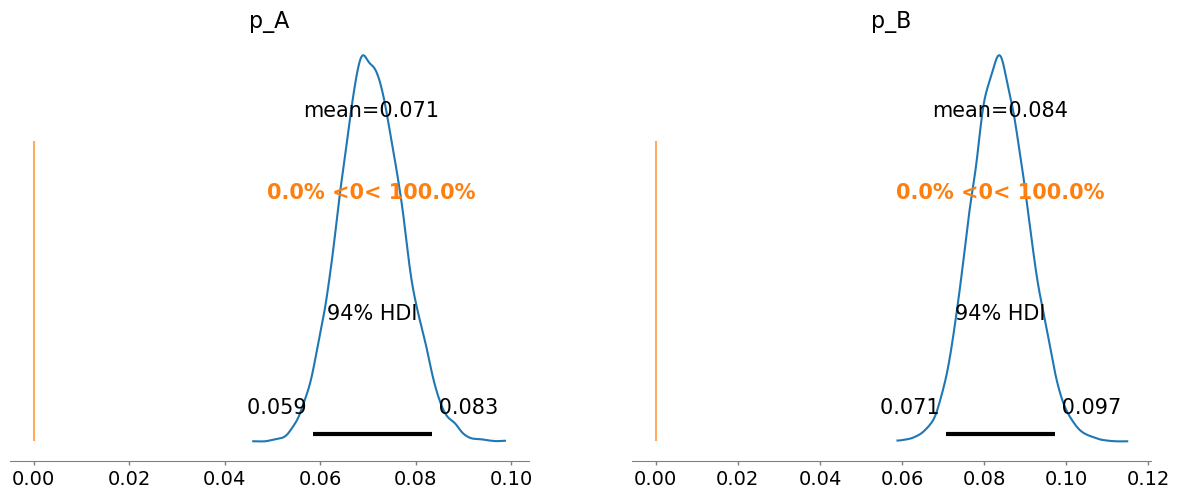
Estimate the posterior distributions of the metrics of interest (like conversion rates) directly, rather than relying on p-values from hypothesis testing.

import pymc as pm
import arviz as az

# Number of visitors
n_A = 1500 # Control
n_B = 1500 # Treatment

# Number of conversions
conversions_A = 105  
conversions_B = 125

with pm.Model() as model:
    # Prior distributions for probabilities of conversion
    p_A = pm.Beta('p_A', alpha=2, beta=10)
    p_B = pm.Beta('p_B', alpha=2, beta=10)

    # Likelihood functions
    obs_A = pm.Binomial('obs_A', n=n_A, p=p_A, observed=conversions_A)
    obs_B = pm.Binomial('obs_B', n=n_B, p=p_B, observed=conversions_B)

    # Sample from the posterior
    trace = pm.sample(5000, progressbar=False, return_inferencedata=True)

# Plotting the posterior distributions with reference line at 0
az.plot_posterior(trace, var_names=['p_A', 'p_B'], ref_val=0)

# Calculate the probability that B is better than A
prob_B_better_than_A = np.mean(trace.posterior['p_B'].values > trace.posterior['p_A'].values)
print(f"Probability that B is better than A: {prob_B_better_than_A:.2f}")

Auto-assigning NUTS sampler...
Initializing NUTS using jitter+adapt_diag...
Multiprocess sampling (4 chains in 4 jobs)
NUTS: [p_A, p_B]
Sampling 4 chains for 1_000 tune and 5_000 draw iterations (4_000 + 20_000 draws total) took 2 seconds.

Probability that B is better than A: 0.92

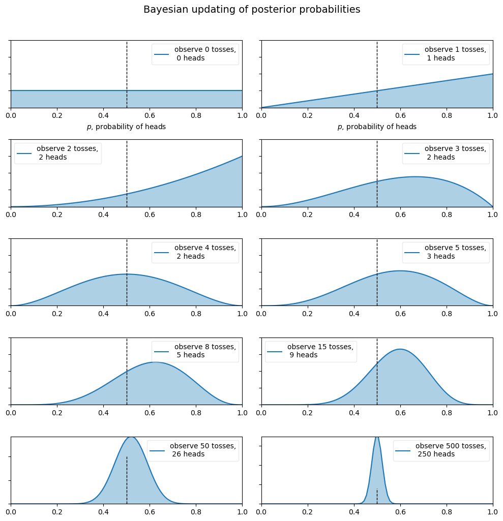
../_images/d2dfa4ed4c75da3c2905e8acbe198b06334084df2e8b27f2dd00efd9cb3f24ee.png

Example from Probabilistic Programming and Bayesian Methods for Hackers

dist = stats.beta
n_trials = [0, 1, 2, 3, 4, 5, 8, 15, 50, 500]
data = stats.bernoulli.rvs(0.5, size=n_trials[-1])
x = np.linspace(0, 1, 100)

plt.figure(figsize=(10, 10))
for k, N in enumerate(n_trials):
    sx = plt.subplot(len(n_trials) // 2, 2, k + 1)
    plt.xlabel("$p$, probability of heads") if k in [0, 1] else None
    plt.setp(sx.get_yticklabels(), visible=False)
    heads = data[:N].sum()
    y = dist.pdf(x, 1 + heads, 1 + N - heads)
    plt.plot(x, y, label="observe %d tosses,\n %d heads" % (N, heads))
    plt.fill_between(x, 0, y, color="#348ABD", alpha=0.4)
    plt.vlines(0.5, 0, 4, color="k", linestyles="--", lw=1)
    leg = plt.legend()
    leg.get_frame().set_alpha(0.4)
    plt.autoscale(tight=True)

plt.suptitle("Bayesian updating of posterior probabilities", y=1.02, fontsize=14)
plt.tight_layout()

../_images/43b211c0e7565f82f3787193de813f23ede73e6cd1547956b29c97b67114cd32.png

Data Distribution Tests#

Shapiro-Wilk Test (Normal Distributions) #

Purpose: It checks how well the data conforms to a normal distribution. More powerful than the K-S test in detecting departures from normality, particularly for small to moderate sample sizes (typically less than 50 samples, though it can be used up to 2000).

Kolmogorov-Smirnov Test #

Purpose: Used to compare a sample with a reference probability distribution (which can be, but is not limited to, a normal distribution). It tests whether two samples are drawn from the same distribution or to compare a sample with a theoretical distribution such as the normal distribution. Generally, the K-S test is considered reliable for larger samples.

sample_size = 1000
data = rng.standard_normal(sample_size)

# Shapiro-Wilk Test for normality
shapiro_test_stat, shapiro_p_value = stats.shapiro(data)
print(f"Shapiro-Wilk: p-value = {shapiro_p_value:0.04f}")

# Kolmogorov-Smirnov Test comparing sample data to a normal distribution
ks_test_stat, ks_p_value = stats.kstest(data, 'norm', args=(data.mean(), data.std()))
# ks_test_stat, ks_p_value = stats.kstest(data, stats.norm.cdf)
print(f"Kolmogorov-Smirnov: p-value = {ks_p_value:0.04f}")

Shapiro-Wilk: p-value = 0.7296
Kolmogorov-Smirnov: p-value = 0.8344

Kullback–Leibler divergence #

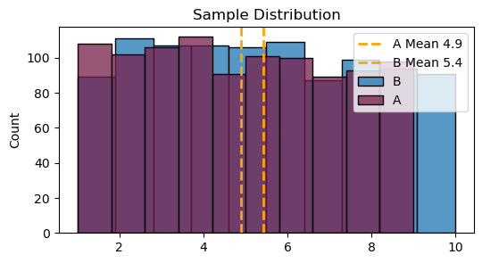
Purpose: Measures how one probability distribution is different from a second.

Not typically used for data distribution tests for a few reasons:

Doesn’t offer a probabilistic interpretation or a hypothesis test framework like p-values.
The first distribution \(P\) must be continuous with respect to the second distribution \(𝑄\). \(P\) can only be non-zero where \(Q\) is non-zero or the KL divergence will be undefined or infinite.
Not symmetric \( D_{KL}(P | Q) ≠ D_{KL}(Q | P) \)

A = rng.uniform(low=1, high=9, size=sample_size)
B = rng.uniform(low=1, high=10, size=sample_size)
p = A + 1e-10  # adding small value to avoid division by zero
q = B + 1e-10  # adding small value to avoid division by zero
kl_divergence = stats.entropy(p, q)
print(f"Kullback-Leibler Divergence: {kl_divergence:0.04f}")

# Alternatively, using histograms
hist_p, bin_edges = np.histogram(p, bins=100, density=True)
hist_q, _ = np.histogram(q, bins=100, density=True)
kl_divergence_hist = stats.entropy(hist_p, hist_q)
print(f"Kullback-Leibler Divergence (histogram method): {kl_divergence_hist:0.04f}")

plt.figure(figsize=(6, 3))
sns.histplot(B, bins=10, color='#1f77b4', label='B')
sns.histplot(A, bins=10, color='#771f4b', label='A')
plt.axvline(x=A.mean(), color='orange', linestyle='--', linewidth=2, label=f'A Mean {A.mean():.01f}')
plt.axvline(x=B.mean(), color='orange', linestyle='--', linewidth=2, label=f'B Mean {B.mean():.01f}')
plt.title('Sample Distribution')
plt.legend()
plt.show()

Kullback-Leibler Divergence: 0.2484
Kullback-Leibler Divergence (histogram method): 0.1083

../_images/a70661a37109f542947c07c6901446b4a90de35acdf09a80d02fa68f85c4c11e.png

Simpson’s Paradox #

Describes a situation where a trend appears in groups of data, but changes when the groups are combined.

Example#

We run an experiment on two days. The first day we apply the treatment to 1% of users and the next day to 50% of users.

The treatment has a better success rate on both days, but when we average the result, it is worse overall due to to weighted averaging.

rng = np.random.default_rng(42) # Setting a seed so it's reproducable

def run_experiment(p, num_simulations):
    successes = rng.binomial(n=1, p=p, size=num_simulations).sum()
    failures = num_simulations - successes
    success_list.append(successes)
    failure_list.append(failures)

success_list = []
failure_list = []

# Day 1: 1% Treatment
run_experiment(p=0.62, num_simulations=500)
run_experiment(p=0.57, num_simulations=9500)

# Day 2: 50% Treatment
run_experiment(p=0.5, num_simulations=5000)
run_experiment(p=0.45, num_simulations=5000)

df = pd.DataFrame({
    "Treatment or Control": ["Treatment", "Control", "Treatment", "Control"],
    "Day of Test": ["Day 1", "Day 1", "Day 2", "Day 2"],
    "Success": success_list, 
    "Failure": failure_list
})

df['Rate'] = (100 * df['Success'] / (df['Success'] + df['Failure'])).round(0)
print("Daily Results:")
display(df)

Daily Results:

	Treatment or Control	Day of Test	Success	Failure	Rate
0	Treatment	Day 1	308	192	62.0
1	Control	Day 1	5463	4037	58.0
2	Treatment	Day 2	2522	2478	50.0
3	Control	Day 2	2301	2699	46.0

print("\nAverage Results:")
df.drop("Day of Test", axis=1, inplace=True)
grouped_df = df.groupby('Treatment or Control').sum()
grouped_df['Rate'] = (100 * grouped_df['Success'] / (grouped_df['Success'] + grouped_df['Failure'])).round(0)
grouped_df

Average Results:

	Success	Failure	Rate
Treatment or Control
Control	7764	6736	54.0
Treatment	2830	2670	51.0

References#

Analysis of Variance - Wikiversity

[man]

Mann-whitney u-test. https://sites.utexas.edu/sos/guided/inferential/numeric/onecat/2-groups/independent/u-test/. Accessed: 2025-01-30.

[Coh94]

Jacob Cohen. The earth is round (p < .05). American Psychologist, 49(12):997–1003, 1994.

[KS25]

Mark A. Kohn and Janet Senyak. Sample size calculators. \textit UCSF CTSI Website, 2025. Available at https://www.sample-size.net/ [Accessed 30 January 2025].