Scaling

There are several different scalers to choose from. Each with their own pros/cons. Using sklearn’s functions:

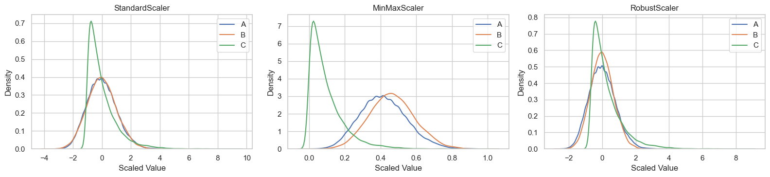
StandardScaler() (Z-score Normalization) removes the mean and scales to the unit variance.

\[ \frac{X_i - X_{Mean}}{X_{StandardDeviation}} \]

MinMaxScaler() brings all values into the range [0, 1]. Maintains the original distribution and relationships between data points.

\[ \frac{X_i - X_{Min}}{X_{Max} - X_{min}} \]

RobustScaler() is robust to outliers.

\[ \frac{X_i - X_{Med}}{IQR} \]

Which to use?

“For most cases, StandardScaler is the scaler of choice. If you know that you have some outliers, go for the RobustScaler.” \(^1\)

Both StandardScaler and MinMaxScaler are very sensitive to the presence of outliers.

Examples

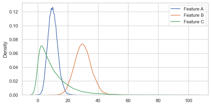
First, we’ll generate three features from different distributions.

import warnings
import numpy as np
import seaborn as sns
import matplotlib.pyplot as plt
from sklearn.preprocessing import StandardScaler, MinMaxScaler, RobustScaler, QuantileTransformer

warnings.simplefilter(action='ignore', category=FutureWarning)
plt.rcParams['figure.figsize'] = (8, 4)

n_samples = 10000
rng = np.random.default_rng(seed=42)

# a = rng.normal(loc=20, scale=10, size=n_samples)
a = rng.poisson(lam=10, size=n_samples)
b = rng.poisson(lam=30, size=n_samples)
c = rng.exponential(scale=10, size=n_samples)

sns.kdeplot(a, label='Feature A')
sns.kdeplot(b, label='Feature B')
sns.kdeplot(c, label='Feature C')
plt.legend()
plt.show()

fig, axs = plt.subplots(1, 3, figsize=(16, 4))

sns.kdeplot(StandardScaler().fit_transform(a.reshape(-1, 1)).ravel(), ax=axs[0], label='A')
sns.kdeplot(StandardScaler().fit_transform(b.reshape(-1, 1)).ravel(), ax=axs[0], label='B')
sns.kdeplot(StandardScaler().fit_transform(c.reshape(-1, 1)).ravel(), ax=axs[0], label='C')
axs[0].legend()
axs[0].set_title("StandardScaler")

sns.kdeplot(MinMaxScaler().fit_transform(a.reshape(-1, 1)).ravel(), ax=axs[1], label='A')
sns.kdeplot(MinMaxScaler().fit_transform(b.reshape(-1, 1)).ravel(), ax=axs[1], label='B')
sns.kdeplot(MinMaxScaler().fit_transform(c.reshape(-1, 1)).ravel(), ax=axs[1], label='C')
axs[1].legend()
axs[1].set_title("MinMaxScaler")

sns.kdeplot(RobustScaler().fit_transform(a.reshape(-1, 1)).ravel(), ax=axs[2], label='A')
sns.kdeplot(RobustScaler().fit_transform(b.reshape(-1, 1)).ravel(), ax=axs[2], label='B')
sns.kdeplot(RobustScaler().fit_transform(c.reshape(-1, 1)).ravel(), ax=axs[2], label='C')
axs[2].legend()
axs[2].set_title("RobustScaler")

for ax in axs:
    ax.set_xlabel("Scaled Value")
    ax.set_ylabel("Density")

plt.tight_layout(rect=[0, 0, 1, 0.95])
plt.show()

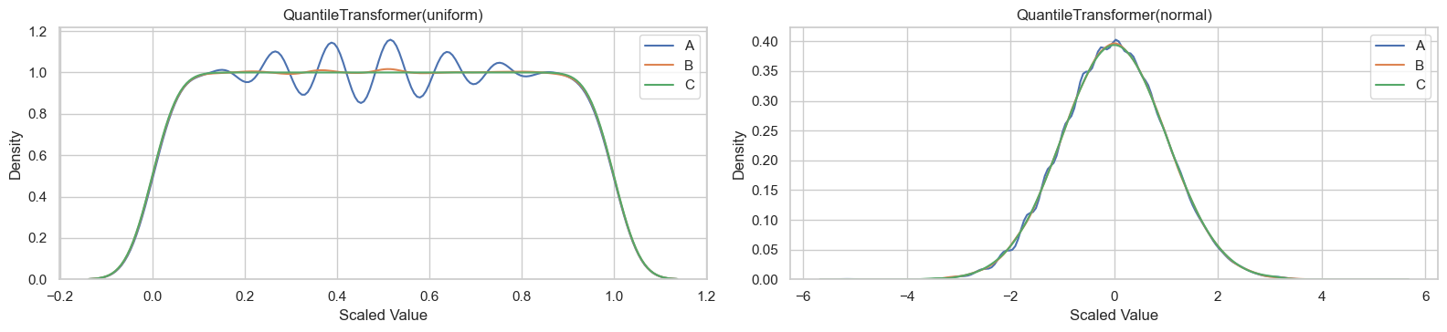
QuantileTransformer()

fig, axs = plt.subplots(1, 2, figsize=(16, 4))

sns.kdeplot(QuantileTransformer().fit_transform(a.reshape(-1, 1)).ravel(), ax=axs[0], label='A')
sns.kdeplot(QuantileTransformer().fit_transform(b.reshape(-1, 1)).ravel(), ax=axs[0], label='B')
sns.kdeplot(QuantileTransformer().fit_transform(c.reshape(-1, 1)).ravel(), ax=axs[0], label='C')
axs[0].legend()
axs[0].set_title("QuantileTransformer(uniform)")

sns.kdeplot(QuantileTransformer(output_distribution='normal').fit_transform(a.reshape(-1, 1)).ravel(), ax=axs[1], label='A')
sns.kdeplot(QuantileTransformer(output_distribution='normal').fit_transform(b.reshape(-1, 1)).ravel(), ax=axs[1], label='B')
sns.kdeplot(QuantileTransformer(output_distribution='normal').fit_transform(c.reshape(-1, 1)).ravel(), ax=axs[1], label='C')
axs[1].legend()
axs[1].set_title("QuantileTransformer(normal)")

for ax in axs:
    ax.set_xlabel("Scaled Value")
    ax.set_ylabel("Density")

plt.tight_layout(rect=[0, 0, 1, 0.95])
plt.show()

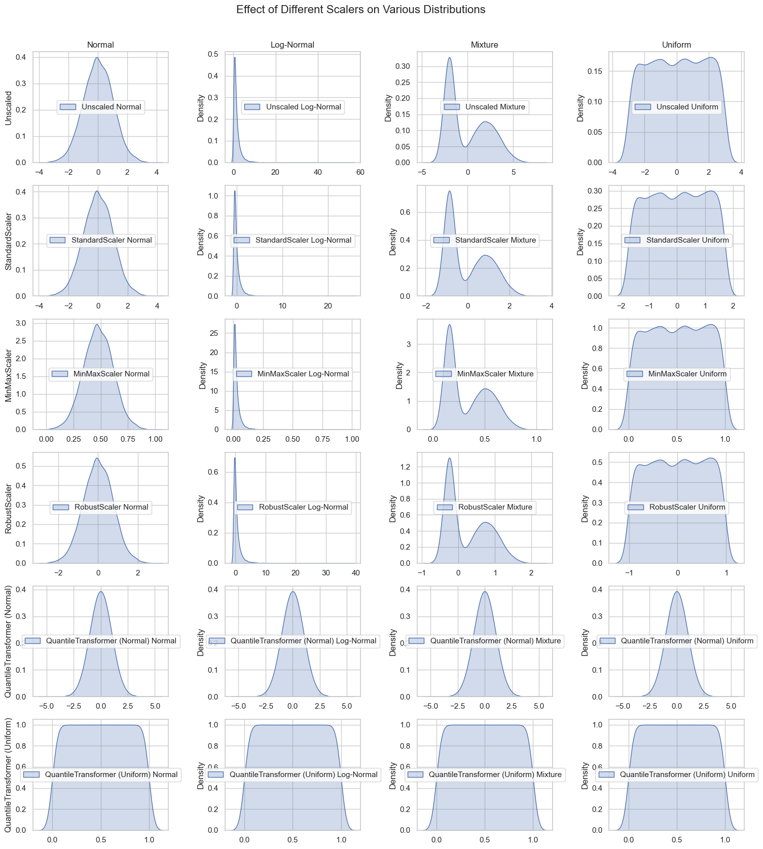
Scalers vs Distributions

sns.set_theme(style="whitegrid")

distributions = {
    "Normal": rng.normal(loc=0, scale=1, size=n_samples),
    "Log-Normal": rng.lognormal(mean=0, sigma=1, size=n_samples),
    "Mixture": np.concatenate([
                rng.normal(loc=-2, scale=0.5, size=n_samples // 2),
                rng.normal(loc=2, scale=1.5, size=n_samples // 2)
            ]),
    "Uniform": rng.uniform(low=-3, high=3, size=n_samples),
}
scalers = [
    ("Unscaled", None),
    ("StandardScaler", StandardScaler()),
    ("MinMaxScaler", MinMaxScaler()),
    ("RobustScaler", RobustScaler()),
    ("QuantileTransformer (Normal)", QuantileTransformer(output_distribution='normal')),
    ("QuantileTransformer (Uniform)", QuantileTransformer(output_distribution='uniform')),
]

n_rows = len(scalers)
n_cols = len(distributions)
fig, axs = plt.subplots(n_rows, n_cols, figsize=(4 * n_cols, 3 * n_rows))

# Iterate over scalers and distributions to plot
for row_idx, (scaler_name, scaler) in enumerate(scalers):
    for col_idx, (dist_name, data) in enumerate(distributions.items()):
        ax = axs[row_idx, col_idx] if n_rows > 1 else axs[col_idx]
        data = data.reshape(-1, 1)
        
        # Apply scaler if not unscaled
        scaled_data = scaler.fit_transform(data) if scaler is not None else data
        sns.kdeplot(scaled_data.ravel(), ax=ax, label=f'{scaler_name} {dist_name}', shade=True)
        ax.legend(loc='center')
        # Set title for the top row
        if row_idx == 0:
            ax.set_title(dist_name, fontsize=12)
        
        # Set ylabel for the first column
        if col_idx == 0:
            ax.set_ylabel(scaler_name, fontsize=12)
        
plt.tight_layout(rect=[0.05, 0.05, 1, 0.95])
plt.suptitle('Effect of Different Scalers on Various Distributions', fontsize=16)
plt.show()