Distributions

A collection of commonly used distributions and their properties.

Discrete Distributions

Discrete distributions describe the likelihood of outcomes for discrete random variables, which can only take on a finite or countably infinite number of distinct values.

Bernoulli Distribution

Example: Coin toss, heads (success) or tails (failure).

Binary, boolean output: 1 (success) with probability p, or 0 (failure) with probability q=1-p.

• Mean: \(p\)

• Variance: \(pq\)

import numpy as np
import seaborn as sns
import matplotlib.pyplot as plt
import scipy.stats as stats
import warnings

warnings.filterwarnings('ignore')

plt.rcParams['figure.figsize'] = (8, 4)
rng = np.random.default_rng(seed=42)
num_simulations = 10000

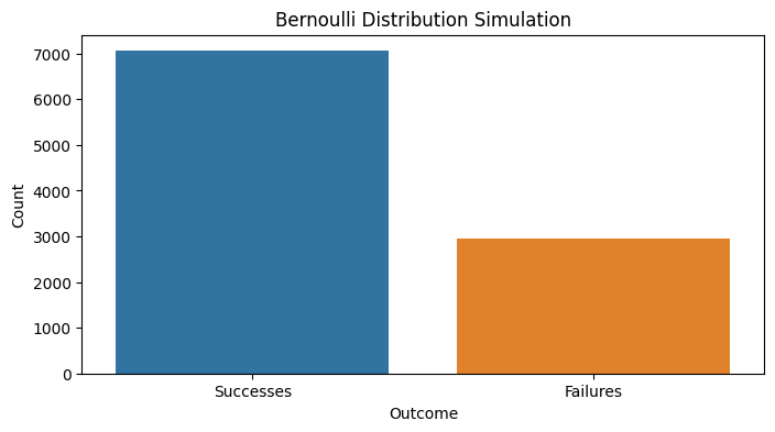
p = 0.7 # probability of getting a "success"
simulations = rng.binomial(n=1, p=p, size=num_simulations)
successes = np.count_nonzero(simulations == 1)
failures = np.count_nonzero(simulations == 0)
print(f'Successes: {successes}, Failures: {failures}')

sns.barplot(x=['Successes', 'Failures'], y=[successes, failures], palette=['#1f77b4', '#ff7f0e'])
plt.xlabel('Outcome')
plt.ylabel('Count')
plt.title('Bernoulli Distribution Simulation')
plt.show()

Successes: 7058, Failures: 2942

Binomial Distribution

Number of successful Bernoulli trials in a sequence.

Example: Calculating the probability of getting a specific number of heads in a fixed number of coin tosses.

Online Calculator

Parameters:

• n: # of successes in a sequence of independent experiments, each asking a yes–no question

• x: # of times for a specific outcome within n trials

• p: probability of success or failure

• q: probability of failure (1-p)

Properties:

• Formula: \({n \choose x} p^x q^{n-x}\)

• Mean: \(np\)

• Variance: \(npq\)

fig, axs = plt.subplots(1, 2, figsize=(12, 4))

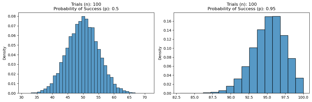
n = 100 # number of trials
p = 0.5 # probability of getting a "success" (heads)
simulations = rng.binomial(n=n, p=p, size=num_simulations)
plot_settings = {'bins': len(np.unique(simulations)), 'color': '#1f77b4', 'stat': 'density'}
sns.histplot(simulations, ax=axs[0], **plot_settings)
axs[0].set_title(f'Trials (n): {n}\nProbability of Success (p): {p}')

n = 100 # number of trials
p = 0.95 # probability of getting a "success" (heads)
simulations = rng.binomial(n=n, p=p, size=num_simulations)
plot_settings = {'bins': len(np.unique(simulations)), 'color': '#1f77b4', 'stat': 'density'}
sns.histplot(simulations, ax=axs[1], **plot_settings)
axs[1].set_title(f'Trials (n): {n}\nProbability of Success (p): {p}')
plt.tight_layout()
plt.show()

Negative Binomial Distribution

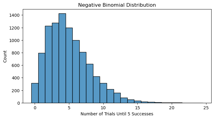
Modeling the number of failed attempts before achieving a specified number of successes in a process.

Example: Determining the number of days until a certain number of people have been infected in a disease outbreak.

FFFSSFS = NegBin(3,p)=7

\( f(y) = \binom{k + r - 1}{k} q^{y - r} p^r \), where \(y = r, r + 1, \ldots\) Properties:

• Mean: \( \frac{r}{p} \)

• Variance: \( \frac{qr}{p^2} \)

r = 5 # number of successes
p = 0.5 # probability of getting a "success" (heads)
simulations = rng.negative_binomial(n=r, p=p, size=num_simulations)

sns.histplot(simulations, color='#1f77b4', discrete=True)
plt.xlabel('Number of Trials Until {} Successes'.format(r))
plt.ylabel('Count')
plt.title('Negative Binomial Distribution')
plt.show()

Geometric Distribution

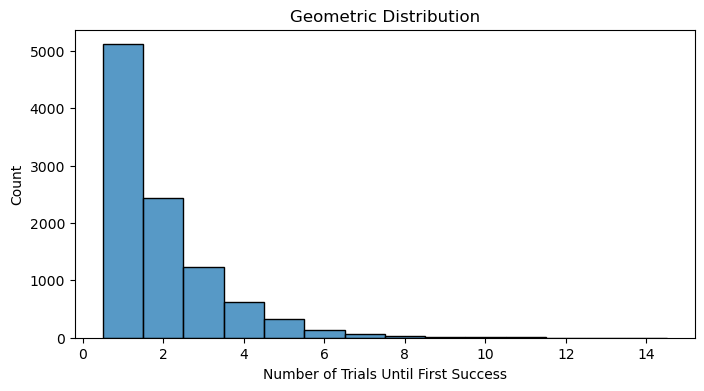
Number of Bernoulli trials until a success. This is a special case of the negative binomial distribution looking for the number of trials until the first success.

Example: Finding the probability that a customer will have to call a certain number of times before their issue is resolved.

Properties:

• Mean: \( \frac{1}{p} \)

• Variance: \(\frac{q}{p^2} \)

p = 0.5 # probability of getting a "success" (heads)
simulations = rng.geometric(p=p, size=num_simulations)

sns.histplot(simulations, color='#1f77b4', discrete=True)
plt.xlabel('Number of Trials Until First Success')
plt.ylabel('Count')
plt.title('Geometric Distribution')
plt.show()

Poisson Distribution

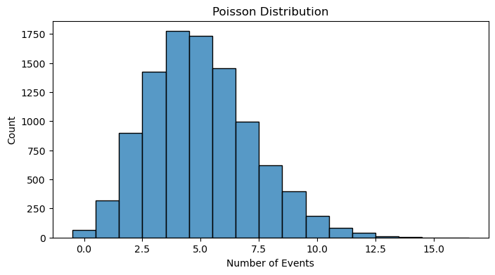
Example: Estimating the number of incoming calls to a call center in a fixed time period.

\( f(x) = \frac{\lambda^x e^{-\lambda}}{x!} \)

\( F(x) = e^{-\lambda} \sum_{i=0}^{x} \frac{\lambda^i}{i!} \)

Properties:

• Mean: \( \lambda \)

• Variance: \( \lambda \)

Eg. Pois(12), What is the prob of exactly 8? (use pmf) 128*e-12/8! =6.55%

lam = 5 # lambda - average rate of success (events per interval)
simulations = rng.poisson(lam=lam, size=num_simulations)

sns.histplot(simulations, color='#1f77b4', discrete=True)
plt.xlabel('Number of Events')
plt.ylabel('Count')
plt.title('Poisson Distribution')
plt.show()

Continuous Distributions

Normal Distribution

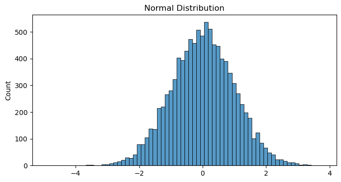
Example: Modeling the distribution of scores on standardized tests such as the SAT.

All you need to know about Gaussian distribution is a great dive into the topic.

mu = 0 # mean
sigma = 1 # standard deviation
simulations = rng.normal(loc=mu, scale=sigma, size=num_simulations)

sns.histplot(simulations, color='#1f77b4')
plt.ylabel('Count')
plt.title('Normal Distribution')
plt.show()

Log-Normal Distribution

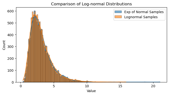
The Log-Normal distribution effectively models data that grows exponentially or has multiplicative rather than additive effects. If a random variable \(X\) is log-normally distributed, then \(Y = ln(X)\) has a normal distribution.

Example: Average call time at a call center.

Fun fact: You can get a log-normal distribution by exponentiating the normal distribution.

mu = 1
sigma = 0.5
normal_samples = rng.normal(loc=mu, scale=sigma, size=num_simulations)
log_normal_samples_direct = rng.lognormal(mean=mu, sigma=sigma, size=num_simulations)

sns.histplot(np.exp(normal_samples), color='#1f77b4', kde=True, label='Exp of Normal Samples', alpha=0.6)
sns.histplot(log_normal_samples_direct, color='#ff7f0e', kde=True, label='Lognormal Samples', alpha=0.6)
plt.xlabel('Value')
plt.ylabel('Count')
plt.title('Comparison of Log-normal Distributions')
plt.legend()
plt.show()

Cauchy distribution

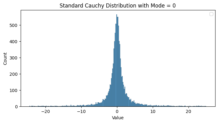
Characterized by its heavy tails and undefined moments. It violates the law of large numbers since the sample mean of iid Cauchy variables does not converge to a finite value as the sample size increases.

The standard Cauchy distribution is a special case of the Student’s t-distribution with one degree of freedom.

Due to the undefined mean and variance, traditional statistical measures like the sample mean and variance are not reliable estimators for the Cauchy distribution. Alternative measures, such as the sample median and interquartile range, are more appropriate.​

The sum of two independent Cauchy-distributed variables is also Cauchy-distributed.

It is used in modeling phenomena where large deviations are more common than predicted by Gaussian models.

standard_cauchy = rng.standard_cauchy(size=num_simulations)
print(f"Limiting the graph to be between (-25, 25), but the actual sample includes values between ({np.min(standard_cauchy):0.2f}, {np.max(standard_cauchy):0.2f})")
standard_cauchy = standard_cauchy[(standard_cauchy > -25) & (standard_cauchy < 25)]

sns.histplot(standard_cauchy, color='#1f77b4')
plt.xlabel('Value')
plt.ylabel('Count')
plt.title('Standard Cauchy Distribution with Mode = 0')
plt.legend()
plt.show()

Limiting the graph to be between (-25, 25), but the actual draws include values between (-2329.17, 2207.21)

Chi-squared distribution

Used primarily in hypothesis testing, and to a lesser extent for confidence intervals for population variance when the underlying distribution is normal. Not as often applied in the direct modeling of natural phenomena.

Goodness of Fit Test: Checking how well observed data fit a theoretical distribution.

Independence Test: Testing for independence between two categorical variables in a contingency table.

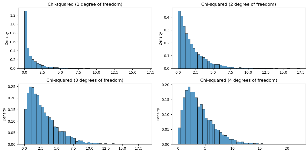
\( \chi^2 = \sum_{i=1}^{k} Z_i^2 \)

Where \( Z_1^2, ..., Z_k^2 \) are standard normal random variables and \(k\) is “degrees of freedom”

Z_1 = rng.standard_normal(num_simulations)**2
Z_2 = rng.standard_normal(num_simulations)**2
Z_3 = rng.standard_normal(num_simulations)**2
Z_4 = rng.standard_normal(num_simulations)**2

plot_settings = {'bins': 50, 'color': '#1f77b4', 'stat': 'density'}
fig, axs = plt.subplots(2, 2, figsize=(12, 6))
sns.histplot(Z_1, ax=axs[0, 0], **plot_settings)
axs[0, 0].set_title('Chi-squared (1 degree of freedom)')

sns.histplot(Z_1 + Z_2, ax=axs[0, 1], **plot_settings)
axs[0, 1].set_title('Chi-squared (2 degree of freedom)')

sns.histplot(Z_1 + Z_2 + Z_3, ax=axs[1, 0], **plot_settings)
axs[1, 0].set_title('Chi-squared (3 degrees of freedom)')

sns.histplot(Z_1 + Z_2 + Z_3 + Z_4, ax=axs[1, 1], **plot_settings)
axs[1, 1].set_title('Chi-squared (4 degrees of freedom)')

plt.tight_layout()
plt.show()

Uniform Distribution

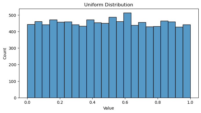
Example: Rolling a dice.

low = 0 # lower boundary of the output interval
high = 1 # upper boundary of the output interval
simulations = rng.uniform(low=low, high=high, size=num_simulations)

sns.histplot(simulations, color='#1f77b4')
plt.xlabel('Value')
plt.ylabel('Count')
plt.title('Uniform Distribution')
plt.show()

Gamma distribution

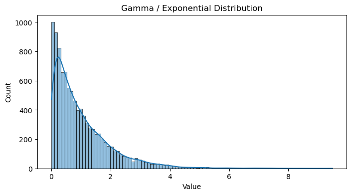
Positive and skewed distributions. Great for modeling the time between events like wait times, failure times, or rainfall.

Commonly used in Bayesian analysis.

scale = 1 # scale parameter (1 / lambda)
simulations = rng.gamma(shape=1, scale=scale, size=num_simulations)

sns.histplot(simulations, color='#1f77b4', kde=True)
plt.xlabel('Value')
plt.ylabel('Count')
plt.title('Gamma / Exponential Distribution')
plt.show()

Exponential Distribution

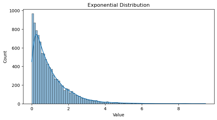
Modeling the time between events in a Poisson process, such as the time between arrivals of customers at a bank.

Example: Estimating the time until failure for electronic components that have a constant failure rate over time.

The exponential distribution is a special case of the gamma Distribution with a shape parameter 1.

scale = 1 # scale parameter (1 / lambda)
simulations = rng.exponential(scale=scale, size=num_simulations)

sns.histplot(simulations, color='#1f77b4', kde=True)
plt.xlabel('Value')
plt.ylabel('Count')
plt.title('Exponential Distribution')
plt.show()

Tweedie Distribution

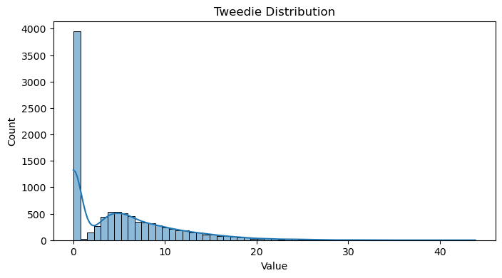
A special case of an exponential distribution with a mass of data at zero.

The code comes from thequackdaddy’s tweedie package. I just took the relevant parts to generate random variables so I did not have to install the whole package.

Show code cell source Hide code cell source

def est_kappa(mu, p):
    kappa = np.where(
        p == 2,
        np.log(mu),
        mu ** (2 - p) / (2 - p)
    )
    return kappa

def est_gamma(phi, p, mu):
    mu = np.array(mu, dtype=float)
    return phi * (p - 1) * mu ** (p - 1)

def rvs(p, mu, phi, size=1000, random_state=42):
    p = np.array(p, ndmin=1)
    if not (p > 1).all() & (p < 2).all():
        raise ValueError('p only valid for 1 < p < 2')
    rate = est_kappa(mu, p) / phi
    scale = est_gamma(phi, p, mu)
    shape = -(2 - p) / (1 - p)
    N = stats.poisson(rate).rvs(size=size, random_state=random_state)
    mask = N > 0
    if not np.isscalar(scale) and len(scale) == len(mask):
        scale = scale[mask]
    if not np.isscalar(shape) and len(shape) == len(mask):
        shape = shape[mask]

    rvs = stats.gamma(
            a=N[mask] * shape,
        scale=scale).rvs(size=np.sum(mask), random_state=random_state)
    rvs2 = np.zeros(N.shape, dtype=rvs.dtype)
    rvs2[mask] = rvs
    return rvs2

p = 1.15 # Power parameter
mu = 5.0  # Mean
phi = 5.0  # Dispersion parameter

simulations = rvs(p, mu, phi, size=num_simulations)

sns.histplot(simulations, color='#1f77b4', kde=True)
plt.xlabel('Value')
plt.ylabel('Count')
plt.title('Tweedie Distribution')
plt.show()

Mixture Distribution

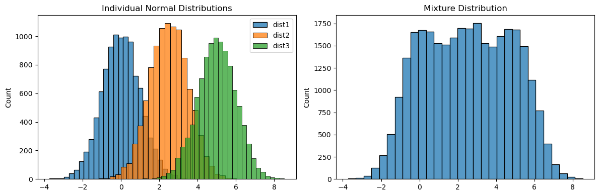
dist1 = rng.normal(loc=0, scale=1, size=num_simulations)
dist2 = rng.normal(loc=2.5, scale=1, size=num_simulations)
dist3 = rng.normal(loc=5, scale=1, size=num_simulations)

fig, axs = plt.subplots(1, 2, figsize=(12, 4))
sns.histplot(dist1, color='#1f77b4', kde=False, ax=axs[0], label='dist1', bins=30)
sns.histplot(dist2, color='#ff7f0e', kde=False, ax=axs[0], label='dist2', bins=30)
sns.histplot(dist3, color='#2ca02c', kde=False, ax=axs[0], label='dist3', bins=30)
axs[0].set_ylabel('Count')
axs[0].set_title('Individual Normal Distributions')
axs[0].legend()

sns.histplot(np.hstack([dist1, dist2, dist3]), color='#1f77b4', kde=False, ax=axs[1], bins=30)
axs[1].set_ylabel('Count')
axs[1].set_title('Mixture Distribution')

plt.tight_layout()
plt.show()

Beta Distribution

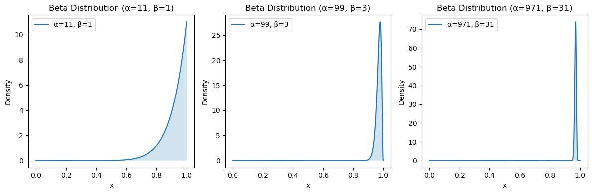
The beta distribution is the conjugate prior probability distribution for the bernoulli, binomial, and negative binomial distributions which makes it uniquely useful in Bayesian statistics.

Here is an example adapted from John Cook’s “A Bayesian view of Amazon Resellers”.

We want to choose the best seller given the following ratings:

• 100% positive out of 10 reviews

• 98% positive out of 100 reviews

• 97% positive out of 1000 reviews

To find the posterior estimate, we add 1 positive and 1 negative review to each.

# Three beta distributions
params = [
    (10, 0), 
    (98, 2), 
    (970, 30)
]
params = [(p[0]+1, p[1]+1) for p in params] # Add 1 every value
x = np.linspace(0, 1, 1000)

fig, axs = plt.subplots(1, 3, figsize=(12, 4))
for i, (a, b) in enumerate(params):
    mean, var, skew, kurt = stats.beta.stats(a, b, moments='mvsk')
    print(f"Beta({a}, {b}) -> Mean: {mean:.03f}, Variance: {var:.03f}, Skewness: {skew:.03f}, Kurtosis: {kurt:.03f}")
    
    y = stats.beta.pdf(x, a, b)
    axs[i].plot(x, y, label=f'α={a}, β={b}')
    axs[i].fill_between(x, y, alpha=0.2)
    axs[i].set_title(f'Beta Distribution (α={a}, β={b})')
    axs[i].set_xlabel('x')
    axs[i].set_ylabel('Density')
    axs[i].legend()

plt.tight_layout()
plt.show()

Beta(11, 1) -> Mean: 0.917, Variance: 0.006, Skewness: -1.553, Kurtosis: 2.977
Beta(99, 3) -> Mean: 0.971, Variance: 0.000, Skewness: -1.087, Kurtosis: 1.699
Beta(971, 31) -> Mean: 0.969, Variance: 0.000, Skewness: -0.342, Kurtosis: 2.734

Then to compare them, we find the probability that a sample from one Beta distribution is greater than a sample from the other Beta distribution.

\(P(X > Y)\) for \(X \sim \text{Beta}(\alpha_1, \beta_1)\) and \(Y \sim \text{Beta}(\alpha_2, \beta_2)\) is:

\( P(X > Y) = \int_0^1 \text{BetaCDF}(y; \alpha_1, \beta_1) \cdot \text{BetaPDF}(y; \alpha_2, \beta_2) \, dy \)

from scipy.integrate import quad

alpha1, beta1 = 99, 3
alpha2, beta2 = 971, 31

def integrand(y):
    return stats.beta.cdf(y, alpha1, beta1) * stats.beta.pdf(y, alpha2, beta2)

result, _ = quad(integrand, 0, 1) # Compute the integral
print(f"The probability that a sample from Beta({alpha1}, {beta1})\n is greater than a sample from Beta({alpha2}, {beta2}) is {result:.3f}")

The probability that a sample from Beta(99, 3)
 is greater than a sample from Beta(971, 31) is 0.403

We can also find an approximate estimate my sampling from the distributions.

size = 100000
b1 = stats.beta.rvs(alpha1, beta1, size=size)
b2 = stats.beta.rvs(alpha2, beta2, size=size)
result = len(b1[b1<b2]) / size
print(f"The probability that a sample from Beta({alpha1}, {beta1})\n is greater than a sample from Beta({alpha2}, {beta2}) is {result:.3f}")

The probability that a sample from Beta(99, 3) is greater than a sample from Beta(971, 31) is 0.404

Alternatively, a sorting algorithm was proposed in Ch. 4 of Bayesian Methods for Hackers.

Central Limit Theorem

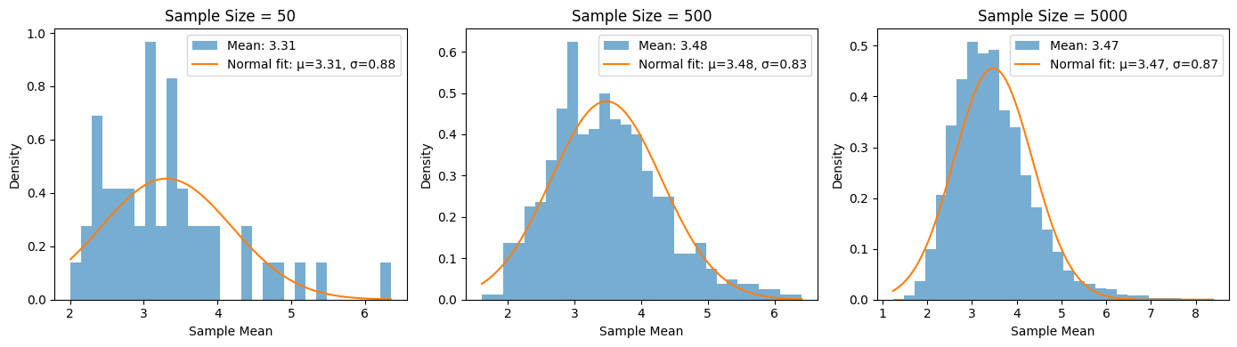
The distribution of sample means approximates a normal distribution as the sample size gets larger, regardless of the population’s distribution.

fig, axs = plt.subplots(1, 3, figsize=(14, 4))
for i, sample_size in enumerate([50, 500, 5000]):
    sample_means = [rng.lognormal(mean=1, sigma=0.7, size=10).mean() for _ in range(sample_size)]
    
    axs[i].hist(sample_means, bins=30, density=True, alpha=0.6, color='tab:blue', label=f'Mean: {np.mean(sample_means):0.02f}')
    
    # Fit and plot a normal distribution to compare
    mu, sigma = np.mean(sample_means), np.std(sample_means)
    x = np.linspace(min(sample_means), max(sample_means), 100)
    axs[i].plot(x, stats.norm.pdf(x, mu, sigma), color='tab:orange', label=f'Normal fit: μ={mu:.2f}, σ={sigma:.2f}')
    
    # Titles and labels
    axs[i].set_title(f'Sample Size = {sample_size}', fontsize=12)
    axs[i].set_xlabel('Sample Mean')
    axs[i].set_ylabel('Density')
    axs[i].legend()

plt.tight_layout()
plt.show()

Statistical Tests for Determining Distribution

Quantile-Quantile Plots (QQ plots)

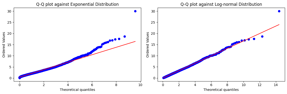
Graphically compares two distributions. Recommended overview: StatQuest - Quantile-Quantile Plots (QQ plots), Clearly Explained!!!

data = rng.lognormal(mean=0.5, sigma=0.7, size=num_simulations)

plt.figure(figsize=(12, 4))

# Exponential Q-Q plot
plt.subplot(1, 2, 1)  # 1 row, 2 columns, 1st plot
stats.probplot(data, dist=stats.expon, plot=plt)
plt.title('Q-Q Plot Comparing Log-Normal Data Versus a Exponential Distribution')

# Log-normal Q-Q plot
plt.subplot(1, 2, 2)  # 1 row, 2 columns, 2nd plot
stats.probplot(data, dist=stats.lognorm(s=0.7), plot=plt)
plt.title('Q-Q Plot Comparing Log-Normal Data Versus a Log-normal Distribution')

plt.tight_layout() 
plt.show()